Much has been said about the relationship between IQ and socioeconomic status (SES). Studies using longitudinal (Strenze, 2007) and within-family designs (Hegelund et al., 2019; Korenman & Winship, 1995; Murray, 2002) suggest a causal effect of general intelligence on SES. Numerous studies have evaluated the predictive validity of IQ relative to factors such as family background (Hernstein & Murray, 1994; Saunders, 1997; Strenze, 2007) and personality (Zisman & Ganzach, 2022). Researchers have partitioned the intelligence-SES correlation into environmental and genetic components using family pedigrees (Rowe et al., 1998) and molecular genetic data (Marioni et al., 2014; Tan et al., 2024). We also know that intelligence shapes SES through occupational sorting—more than 20% of the variation in IQ can be accounted for by between-occupation differences (Gottfredson, 1997; Wolfram, 2023). To date, fourteen meta-analyses have been published on the relationship between measures of cognitive ability and SES (Korous et al., 2022). To clarify the terminology, IQ is a score on a test of cognitive ability, while SES is an academic term for class, which is typically operationalized as an individual’s education, income, occupational status, or a combination of all three.
There are, however, many more cognitive abilities than what is measured by IQ, and we know much less about how they relate to SES. Spearman (1904) showed that cognitive tests exhibit positive correlations, otherwise known as the positive manifold. This implies the existence of a general factor of intelligence (g) which affects performance on all cognitive tests. Thus, an IQ score based on one or more cognitive tests will measure g (Johnson et al., 2004; Spearman, 1927, pp. 197–98). However, cognitive tests also capture domain-specific abilities in addition to g. For example, scores on paragraph comprehension and vocabulary tend to cluster together more so than with other tests, indicating that they capture both g and a specific verbal ability.
After Spearman’s discovery of g and specific abilities, psychologists would use the technique of factor analysis to model performance across tests as combinations of g and specific abilities (Carroll, 1993). Unfortunately, of the little research into how specific abilities affect socioeconomic status, almost all of it uses a crude approach—that of “tilt”, rather than factor analysis. These tilts are difference scores of two abilities—for example, verbal minus mathematical scores—or contrasts of groups of individuals high in one ability versus another.
There are two essential problems with the tilt method. Firstly, if one ability approximates g more closely, a tilt effect may reflect g’s influence rather than specific abilities. Secondly, even if a tilt does not correlate with g, it is impossible to tell which specific ability drives the effect. If doing better on a verbal test than a mathematical one is associated with a higher education later in life, does that imply that the verbal specific ability encourages education or that the mathematical specific ability discourages education? The latter is not implausible if leaving school to work is more attractive with mathematical skills. Tilt studies can only hint at the effects of specific abilities, rather than exactly estimate their influence.
One of the earliest studies in this vein, Gohm, Humphreys, and Yao (1998) used longitudinal data to compare the life outcomes of students who were in the top 1% of spatial ability against those who were in the top 1% of math. The high-spatial group had a lower educational attainment, with 33% leaving education after high school compared to 7% of the high math group. The high spatial group also earned 13% less.
A similar result was found by Edwards et al. (2025), who used scores on verbal and performance IQ from Wechsler Revised Intelligence Scales to predict years of education. Performance IQ includes a block design test that taps into spatial ability. They found that verbal IQ was substantially more predictive of education and income than performance IQ, albeit the difference was not statistically significant for income.
More recent research has focused on comparing mathematical and verbal abilities, with conflicting results. Using longitudinal data, Aucejo and James (2021) found that performance on English exams is much more predictive of college enrollment than math exams. By contrast, Ganzach, Sorjonen, and Pazy (2025) showed that a higher math-versus-verbal tilt in the National Longitudinal Studies of Youth 1979 and 1997 predicted greater education and income.
Ganzach and Patel (2018) studied the effects of cognitive abilities on income using three tests, instead of the usual two typical of the tilt approach. The tests measured literacy, numeracy, and technological problem-solving, the latter of which assessed the ability to use email, websites, and spreadsheets. Besides the first principal component (approximating g), the remaining two components (representing specific abilities) showed negligible associations with income.
Research on how specific abilities relate to occupations has similarly relied on tilt approaches. In the Project Talent dataset, Gohm, Humphreys, and Yao (1998) found that high-spatial students were five times more likely to enter labor occupations and ten times less likely to enter social science fields than their high-math peers. In the same sample (Wai et al., 2009), verbal ability also characterized occupational choices—those working in humanities-related occupations outperformed engineers on verbal performance. Similar results have been found by comparing tilt in highly intelligent people in the Study of Mathematically Precocious Youth (Shea et al., 2001).
Specific abilities and occupations have also been studied using the Armed Services Vocational Aptitude Battery, the same test of cognitive ability used in our study. In the National Longitudinal Studies of Youth, higher performance on tech subtests (like electronic information) predicts having a STEM occupation, while higher performance in verbal subtests (like word knowledge) predicts having a humanities occupation (Coyle, 2018, 2019).
A key limitation of most of the studies linking specific abilities to occupations is their chosen occupational categories. Firstly, few occupational categories are used, resulting in very broad groups. Secondly, these categories track which academic fields are deemed relevant to the job, e.g., social science occupations or fine and performing arts occupations. This approach makes it difficult to pinpoint exactly which occupations are related to specific abilities.
Carretta and Ree (2024) is an exception to this limitation, having used a range of specific occupations, albeit limited to roles within the United States Air Force. The authors calculated a tilt representing general ability minus a composite of the tech subtest. They then measured the average level of tilt for occupations in the United States Air Force. The occupations “weather” and “airfield management” had high scores on the tilt metric, while low scores were found for “tactical aircraft maintenance” and “aerospace propulsion”. This study provides vivid evidence that we sort into occupations based on our cognitive abilities; however, it is important to bear in mind that the Air Force already assigns recruits to jobs based on subtest performance.
Most recently, Giannelis et al. (2025) calculated the genetic correlation between specific quantitative ability (orthogonal to g) and a range of occupations. Although limited in statistical power, the authors found significant positive correlations with being a software analyst or mathematician and negative correlations with being a writer, government official, or trade unionist/NGO organizer.
One explanation for the limited literature relating specific abilities to SES is the popular belief that specific abilities are not very important. As Jensen (1984) once said, “for most jobs, g accounts for all of the significantly predicted variance; other testable ability factors, independent of g, add practically nothing to the predictive validity”. This conclusion was further supported by Ree and Earles (1991), who found that adding specific abilities to regression models of job performance only improved by .01. The authors coined the phrase “not much more than g”. Thirty years on, Ree and Carretta (2022) concluded that the evidence had only strengthened for their position, claiming in the journal Intelligence that specific abilities were “still not much more than g”. Whether an improvement of .01 or .02 is practically meaningful in recruitment is debatable (Schneider & Newman, 2015). However, the claim that specific abilities offer “not much more than g” should not be generalized; in regard to SES and occupational choice, we have little idea of how the predictive validity of specific abilities compares with that of g.
Our study provides a comprehensive analysis of how distinct cognitive abilities shape socioeconomic outcomes. Unlike earlier work that relied on tilt measures, we employed confirmatory factor analysis to pinpoint the precise abilities driving socioeconomic status. To control for shared upbringing, we compared siblings, isolating each ability’s influence on socioeconomic status. We then tracked these effects across the life course to see how their impact changes over time. Finally, by calculating average ability levels across various occupations, we clarified how specific cognitive strengths guide occupational choice.
In light of the widespread skepticism about specific abilities (Ree & Carretta, 2022; Ree & Earles, 1991), perhaps our most important contribution is to clearly quantify their importance. We calculate the ratio of the multiple correlation of specific abilities to the correlation of g with outcomes. That is, we determine how large the effects of specific abilities are relative to the effect of general intelligence. We also quantify the degree to which people sort into occupations by specific abilities, just as has been done with g, allowing the effects to be compared and contrasted.
Understanding the relative importance of different cognitive abilities is of significant policy concern. Today in the United States, similar to other developed nations, children are expected to spend 16 and a half years in education (Global Data Lab, 2024). Such a significant investment of time and money ought to be used efficiently to develop the most useful forms of cognitive ability. Yet today, we have little idea of how specific cognitive abilities impact important life outcomes. Without an understanding of the effects of different cognitive abilities, it is impossible to tailor school curricula to developing the most valuable cognitive skills.
Data
The National Longitudinal Surveys are a series of studies run by the U.S. Bureau of Labor Statistics, created to analyze economic behavior. We used two of these surveys, the National Longitudinal Studies of Youth 1979 and 1997 (NLSY79 & NLSY97), because of their rich cognitive data and their similarity to each other, which allowed for replication across generations. As these are the only National Longitudinal Surveys of Youth, we refer to them collectively as the NLSY.
The NLSY79 recruited 12,686 individuals (aged 14–22 in 1979) using household probability sampling (Bureau of Labor Statistics, 2025a). It consisted of three groups: a representative sample of 9,964 non-incarcerated civilians, an oversample of Hispanic, Black, and economically disadvantaged civilians, and a third group enlisted in the military. The NLSY79 cohort was surveyed annually until 1994, biennially afterward, and is still ongoing today. The oversample was dropped in 1990, and the military sample was dropped in 1984.
The NLSY97 largely mirrored its predecessor (Bureau of Labor Statistics, 2025b), but followed people of the subsequent generation. It sampled 8,984 people, aged 12 to 16 on December 31, 1996. The sample was selected to represent non-incarcerated civilians, but with an oversample of Hispanic and Black individuals. For the sake of simplicity, we did not remove oversamples from either the NLSY79 or NLSY97, and we did not use sampling weights.
Both NLSY79 and NLSY97 sampled households and other dwelling units to identify eligible individuals. This meant that multiple respondents often came from the same household. Multiple survey questions asked about family relationships, allowing the relatedness between participants to be estimated. Rodgers et al. (2016) created a pedigree for NLSY participants and made it available through their NlsyLinks R package. We used this tool to identify all full siblings who share both parents. Within our analysis sample for the NLSY79, there were 1,417 families of two-sibling pairs, and 614 families with three or more siblings. Likewise, the NLSY97 included 1,155 families of two-sibling pairs, and 139 larger families.
Cognitive tests
The Armed Services Vocational Aptitude Battery (ASVAB; Bureau of Labor Statistics, 1982, 2024) is a multiple-choice test. It is used to determine eligibility for the United States Armed Forces and to guide the assignment of recruits. The test was adopted by all branches of the forces in 1976.
The ASVAB was administered to the NLSY79 in 1980 and NLSY97 in 1999 to norm the test (Wallace et al., 2022). Our analysis samples consisted only of individuals in the NLSY79 and NLSY97 who had completed the ASVAB. In the NLSY79, 6% of respondents did not take the ASVAB; in the NLSY97, this figure was 22%. After excluding those individuals, our analysis samples comprised 11,914 (NLSY79) and 7,008 (NLSY97) participants.
The ASVAB was not identical between cohorts. The NLSY97 added the assembling objects subtest, and it separated the auto & shop information subtest into two: the auto information and shop information subtests. The NLSY79 calculated subtest scores from the number of question items answered correctly on a paper-and-pencil test. By contrast, the NLSY97 used a computerized adaptive testing format. Higher-ability respondents received more difficult items, and all scores were estimated via a Bayesian scoring procedure.
We took several steps to ensure the ASVAB is comparable across the surveys. The Assembling Objects test was dropped from the NLSY97. Each test score was residualized on the sex, self-identified ethnicity, and age at which the participants took the test. This ensures that the scores represent performance relative to the test taker’s demographic. The ethnicity categories in the NLSY79 are Hispanic, Black, and White. In the NLSY97, the categories are Black, Hispanic, mixed, and other. A Z-score transformation was applied, so the average score is 0 and the standard deviation is 1. In the NLSY97, we summed Shop Information and Auto Information tests together, after residualizing them separately, and then Z-score transformed to create an Auto & Shop Information test. This approach is sensible since the two subtests include a roughly equal number of items and it is current practice to combine the subtests in the unusual cases that the ASVAB is still administered on paper (Segall, 2004). The ten ASVAB subtests, their abbreviations, and descriptions are in Table 1. Test descriptions are adapted from those given on the ASVAB Fact Sheet (Official ASVAB, 2024).
In addition to the ASVAB, the NLSY79 also contains IQ scores (Bureau of Labor Statistics, 2025c). The administration of the NLSY contacted the high schools of participants to acquire their transcripts. The NLSY79 asked for IQ scores from nine common tests, such as the Stanford Binet and the Lorge-Thorndike test. The high school could also write in performance on any other tests taken. We did not use the write-in data due to some of the unusual or inappropriate tests used, such as aptitude tests for college entrance. Some of the scores were implausibly large or small, so we omitted any values below 70 and above 145. Individuals with more than one IQ score were assigned their average score. We then residualized this average IQ score on ethnicity and age before standardizing it to have a variance of one.
In both NLSY, high school transcripts were used to record performance on aptitude tests (Bureau of Labor Statistics, 2025c, 2025d). The NLSY79 recorded performance on the verbal and mathematical portions of the PSAT, SAT, and ACT. What was recorded as the “verbal ACT” score likely reflects the performance on the ACT English test, since the reading section was added to the ACT in 1989, and the writing section was added in 2005. The NLSY97 similarly recorded performance on the SAT and ACT from high school transcripts. Due to the addition of the reading test, the NLSY97 reported performance on math, English, and reading subtests. The NLSY97 also asked participants for self-reports of their SAT scores. We opted to use the self-reports because they had a larger sample size.
The NLSY97 administered the mathematics subtest of the Peabody Individual Achievement Test (PIAT) to all participants in 9th grade or below during the first survey wave (Bureau of Labor Statistics 2025d). In waves 2–6, only those who were both 12 years old on December 31, 1997 and who had been in 9th grade or below in wave 1 were re-tested; in wave 6, administration was further limited to current high-school students. We standardized each respondent’s PIAT math score within its wave, then averaged these standardized scores across waves, and finally re-standardized the wave-average.
Measures of socioeconomic status
Education is operationalized as the highest grade of education ever reported by a participant, which is precalculated in the NLSY. This measure ranges in value from 0 to 20. Since some individuals might drop out of the study before finishing their education, we set education as missing for any individual who did not participate in the NLSY from the age of 30 onwards. In the NLSY79, 18% of the sample were thus missing a value for education, while 10% were missing in the NLSY97.
During each survey wave, participants were asked for their occupation. The Bureau of Labor Statistics then subsequently transformed their response into an occupation code, as used in a United States census. At certain years, the NLSY would change the occupation codes used. For example, in the 21st century the NLSY79 tracks occupation using 2000 census codes. For consistency in measuring occupational status, in the NLSY79 we only used occupations coded with the 1970s census scheme in the 1979–2000 waves. In the NLSY97, we used occupations coded with the 2000 census codes from waves 2002–2021.
Each occupation was assigned a Duncan socioeconomic index score (SEI; Duncan, 1961). For simplicity, we refer to these scores as occupational status. These scores were created as a weighted average of the income and education level of incumbents in the occupation. The weights are regression coefficients used to predict how prestigious occupations are, as measured with ratings from the public. Our sources for SEI scores also provided prestige measures of occupational status. Our analyses are very similar when using this alternative measure. This is consistent with the fact that different measures of occupational status correlate extremely well (Akimova et al., 2024). The raw results from these analyses can be found on this study’s OSF page.
For the NLSY79, we used SEI scores created for 1970s census codes (Hauser & Featherman, 1977). We used a version of these scores, altered to remove errors, which was developed as part of the Wisconsin Longitudinal Study (1996). For the NLSY97, we used SEI scores developed for use in the Generalized Social Survey with 2010 census codes (Hout et al., 2014). A “crosswalk” from the United States Census Bureau (2011) was used to assign each 2002 census code in the NLSY97 a corresponding 2010 census code. If the 2002 occupation was split into multiple 2010 occupations, we gave it the SEI score of the new occupation with the most similar-sounding name. For example, the 2002 census code 0620 Human Resources, Training, and Labor Relations Specialists was given the 2010 census code 0630 for Human Resources Workers. If the 2002 occupations were combined in the 2010 census code, then they were given the same SEI codes. The conversion we used is available on the study’s OSF page.
To create a composite measure of occupational status, we Z-score transformed occupational status within sample waves, then averaged values across waves before finally Z-score transforming the resulting average. This means that the occupational status composite reflects the status of a participant’s jobs relative to others who were working at the same time. In the NLSY79, 4% of participants and in the NLSY97, 1% were missing data on the occupational status composites.
We performed a similar procedure to create a composite of income. We calculated income, within a survey year, as the sum of self-reported employment, farm, and business income before tax for the prior year. To obtain a variable more normally distributed, we applied the natural logarithm to income within each survey year, leaving individuals with zero income as missing. Using all available data, the income composite in the NLSY79 was calculated annually from the years 1979–2022, although only biennially from 1994 onwards. In the NLSY97, it was calculated from 1997–2021, but biennially from 2011. In both the NLSY samples, 2% of participants were missing a value for the income composite. Reliability metrics and further missingness statistics for the composites are available on the study’s OSF page.
Occupational categories
The sample size of the NLSY is insufficient for analyzing cognitive ability by specific occupations. Thankfully, the U.S. census categorizes jobs hierarchically. For example, in the 1980s occupational classification system, the occupation of physician is part of the minor occupational code of health diagnosing occupations, which in turn is part of the major occupational code of managerial and professional specialty occupations. We used the minor occupational codes to balance sample size against the resolution of the occupation. The minor occupational codes are given in the NLSY codebooks (Bureau of Labor Statistics, 1980, 2002). For simplicity, we refer to the minor occupational codes as occupations.
For analyses of occupation categories, we used participants’ occupation in the tenth survey year (1989 and 2007 for the NLSY79 and NLSY97 respectively). These years were chosen based on sample size and because the participants should have begun their careers ten years after being recruited. To apply appropriate SEI scores, we used the 1970s census codes in the NLSY79; however, for analyzing specific occupations, we used the 1980s census, which presumably better categorizes the occupations of 1989.
We removed all occupations with five or fewer workers in either NLSY, to ensure our estimates were reliable. Of the 70 occupations in our NLSY79, 4 were removed. In the 31 occupations in the NLSY97 sample, one was removed. In terms of participants, out of 8,667 NLSY79 individuals with an occupation code, eight were removed for being in rare occupations. In the NLSY97, two individuals out of 5,172 were removed.
In the appendix, we tested whether cognitive abilities predicted the RIASEC (Realistic, Investigative, Artistic, Social, Enterprising, and Conventional) vocational interests (Holland, 1959) of participants’ occupations. We used version 30.2 of the Occupational Information Network (O*NET) occupational interests (National Center for O*NET Development, 2026; Putka et al., 2023), which were on a 1–7 scale. To develop these ratings, a set of occupations was given RIASEC ratings through expert judgement; then O*NET applied a machine learning approach to predict RIASEC interests for jobs using their title, description, and task statements.
These RIASEC scores are for jobs in the 2018 standard occupational classification (SOC) system. To map the 2002 census codes in the NLSY97 onto SOCs, we applied the 2002–2010 census crosswalk (U.S. Census Bureau, n.d., 2025) and then the 2010–2018 census crosswalk (U.S. Census Bureau, 2019), which also contained the corresponding SOCs. For the 1980s census codes in the NLSY79, we fed the occupation titles into a machine-learning text classifier: The National Institute for Occupational Safety and Health’s Industry and Occupation Computerized Coding System (NIOCCS; National Institute for Occupational Safety and Health, n.d., 2022). The tool then provides a best guess for the closest SOC corresponding to the occupation. When a specific SOC was not in O*NET’s dataset, we applied the RIASEC scores from its SOC family. For example, there was no RIASEC score for secondary school teachers (SOC: 25-2030), so we applied the average scores for occupations in the 25-203X family: Secondary School Teachers, Except Special and Career/Technical Education (SOC: 25-2031) and Career/Technical Education Teachers, Secondary School (SOC: 25-2032). Among participants with an occupation, only a small proportion could not be matched with RIASEC scores (16.2% in NLSY79 and 8.1% in NLSY97).
Method
Factor structure
To determine the number of latent factors of cognitive ability underlying the ASVAB, we applied parallel analysis. To identify these factors, we applied exploratory factor analysis to the ASVAB subtests in the NLSY samples. A bifactor quartimin rotation was used (Jennrich & Bentler, 2011). This criterion prefers solutions where all subtests load on the general intelligence factor and on only one group factor (a specific ability), penalizing cross-loadings. The solutions were calculated using the factanal function from the stats package in R, employing maximum likelihood estimation.
We used the loadings from the exploratory factor analysis to guide the construction of a confirmatory factor analytic model, using the lavaan package in R. To improve interpretability and reduce overfitting, we specified paths only if the corresponding EFA loadings were greater than or equal to .10 in the NLSY79. For ease of comparison, we then applied the same model structure to the NLSY97. To examine whether the models were capturing the same latent variables in both samples, we compared the loadings across samples and tested for metric measurement invariance. We compared a model with freely estimated loadings to one with loadings constrained to be equal across the NLSY samples. We then evaluated the effect of the constraint on the fit by using the change in the root mean squared error of approximation (RMSEA), standardized root mean squared residual (SRMR), and the comparative fit index (CFI).
A key limitation of bifactor models is that they tend to overfit (Bonifay et al., 2017; Markon, 2019; Reise et al., 2016), due to the number of free parameters used. Capitalizing on the chance features of a given sample may undermine the validity of the model’s identified latent variables and reduce the generalizability of our results. We ran several sensitivity tests to our key analyses. Firstly, we tried an additional model in CFA where loadings were fixed to their corresponding loadings in EFA. We referred to this approach as an exploratory structural equation model (ESEM). By allowing for cross-loadings, this approach can even more closely fit the data.
As a second approach, we created bifactor models using a Schmid–Leiman transformation (Schmid & Leiman, 1957). We first fit an oblique CFA with the same lower-order cognitive domains as in our main bifactor analysis. Each subtest was assigned only to its designated lower-order factor; thus, if a subtest was assigned to the Speed specific ability in the exploratory bifactor model, it loaded only on the Speed factor in the higher-order representation. We then modeled the correlations among the lower-order factors with a single higher-order general factor and applied the Schmid–Leiman transformation, yielding the corresponding bifactor representation of that higher-order solution. The value of this approach is that, within each specific ability, subtests cannot take arbitrary combinations of g and specific-ability loadings. Instead, those two loadings are constrained to remain proportional across subtests, which helps limit overfitting.
In the case where the identified latent variables were not valid, generalizable, or comparable across samples, we also repeated several key analyses using principal components. If we could not be confident that we studied the same latent variables across the NLSY samples, then, with principal components, we could at least be sure that we studied the same manifest variables. To aid comparison, we projected the principal component loadings from the NLSY79 into the NLSY97.
Prediction
For prediction, we regressed the indicators of socioeconomic status on latent factors of cognitive ability within structural equation models. This involved adding regression paths to the CFA modelled in lavaan. Control variables included age, sex, and dummy variables for self-identified ethnicity. For the sake of simplicity, missing values were dealt with in all models via listwise deletion. All continuous variables were standardized to have a variance of one, prior to removing participants with missing observations. We clustered the standard errors by family, where family is defined as sharing two biological parents. We defined statistical significance as (Benjamin et al., 2018).
To evaluate the relative importance of specific abilities compared to general intelligence, we report the ratio of their effects. Is the effect of specific abilities 5%, 10%, or 30% as large as the effect of g? Formally, this is the ratio of the multiple correlation between the specific abilities and SES to the simple correlation between g and SES.
Rs/Rg
The correlations are the square roots of the variance explained by specific abilities or g. For ease of notation, we use the capital to denote g’s correlation with the outcome. We avoid reporting variance ratios, because squaring places effects on a squared scale and can make differences in predictive magnitude appear larger than they do on the correlation scale (Del Giudice, 2021; Funder & Ozer, 2019). For example, suppose g explains 36% of the variance and specific abilities explain 4%. On the variance-explained scale, this is a 9:1 ratio. However, the corresponding correlations and differ by a factor of 3. Because our aim is to compare relative predictive magnitude, we report ratios on the correlation scale.
Before taking square roots, we estimated the variance explained by summing the squared regression coefficients of the specific abilities or g. Note that since the ASVAB subtests have been residualized on the control variables and, by design, the latent factors of cognitive ability are orthogonal, each cognitive ability is uncorrelated with every other independent variable. This makes it appropriate to equate the regression coefficient of a cognitive ability to its correlation.
Within-family modeling
Many plausible environmental confounds are shared by siblings, such as parental education, school quality, or any shared aspect of upbringing more generally. To deal with these confounds, we modeled the within and between family variation separately. This involved decomposing an individual’s performance on each ASVAB subtest into the average performance of their siblings (the between-family component) and the deviation of the individual from the sibling average (the within-family component).
xij⏟subtest score =ˉx⋅j⏟between-family component +(xij−ˉx⋅j)⏟within-family component
We fitted a multilevel CFA in lavaan to the within and between-family components, using the same configural model used for individual-level analyses. This assumes that there are the same latent factors of cognitive ability both within and between families, although their loadings on the ASVAB subtests need not be equal. We then ran our prediction model, regressing the latent cognitive abilities on SES. Race was dropped as a control variable since it should have no within-family variance. The same within-between decomposition applied to the ASVAB subtests was also applied to the dependent and control variables.
Occupational modeling
To estimate the average cognitive ability within an occupation, we performed the following regression:
Cognitive abilityki=αkm+βkmOccupationmi+εki
Here, a dummy variable is regressed on a cognitive ability (say general intelligence). The dummy variable takes the value of one when an individual is a member of the occupation (a teacher, for example) and zero otherwise. In this example, the regression slope represents the difference in the average general intelligence between teachers and study participants who are not teachers. For simplicity, we refer to this slope as the average cognitive ability of an occupation.
Because we estimated the cognitive abilities of many occupations, for each cognitive ability we applied a false discovery rate (FDR) correction across occupations. We considered to be significant; this is lower than the standard threshold of in line with our stringent choice of using to denote significance elsewhere.
Usually, the degree of occupational clustering is quantified as the variance of a cognitive ability between occupations as a fraction of the total variance in the cognitive ability. In other words, this is the variance in cognitive ability explained by occupation differences. This statistic was calculated from the model below, regressing each occupation dummy variable (except an omitted reference category) on the cognitive ability simultaneously.
Cognitive abilityki=αk+M−1∑m=1βkmOccupationmi+εki
For clearer communication (Del Giudice, 2021; Funder & Ozer, 2019), we prefer to use the square root of the variance explained: the multiple correlations of occupation on each cognitive ability.
Results
Factor analysis
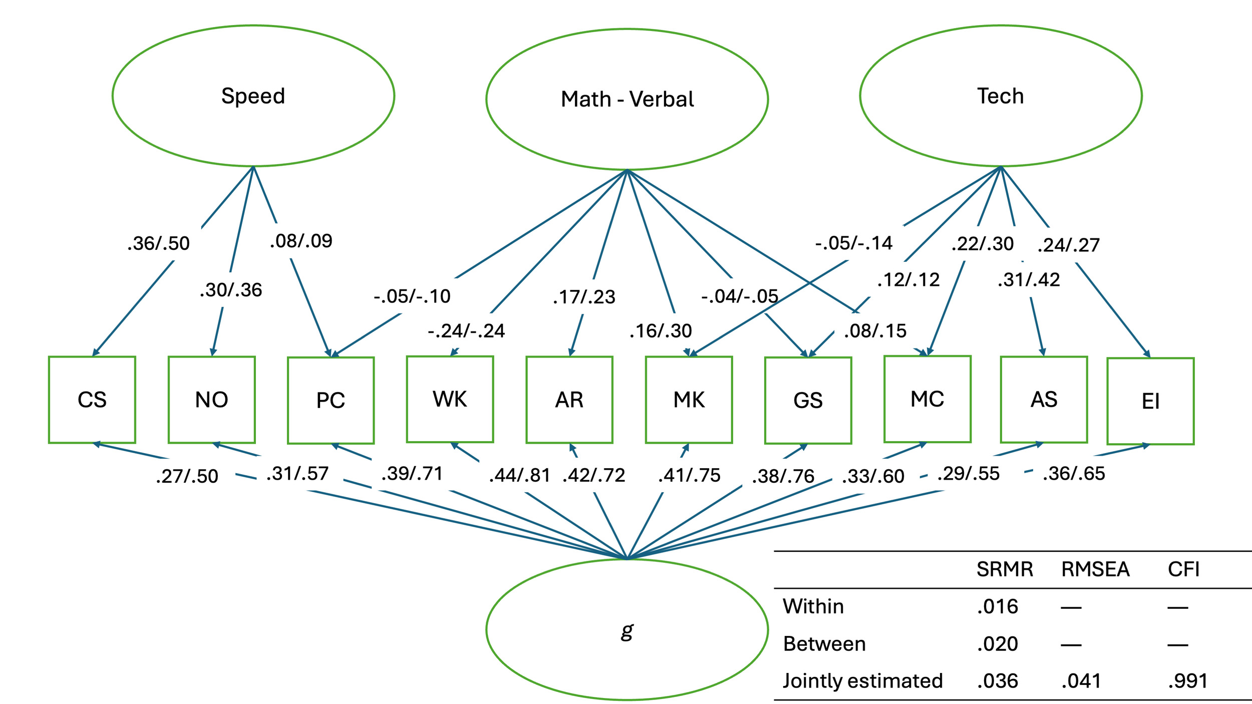
The correlation matrix of the NLSY subtests is shown in Appendix Table A1 and the loadings from the exploratory factor analyses (EFA) are shown in Appendix Table A2. The EFA in the NLSY79 found a general factor of intelligence and three specific abilities, which we label as tech, speed, and the math-verbal factor; the latter was positively associated with math subtests and negatively with verbal tests. The tech factor loaded on those tests related to practical vocational skills, such as electronics information and auto & shop information. In the NLSY97, the tech factor loaded on the same subtests, but math tests positively loaded on the speed factor and showed smaller loadings with the math-verbal factor.
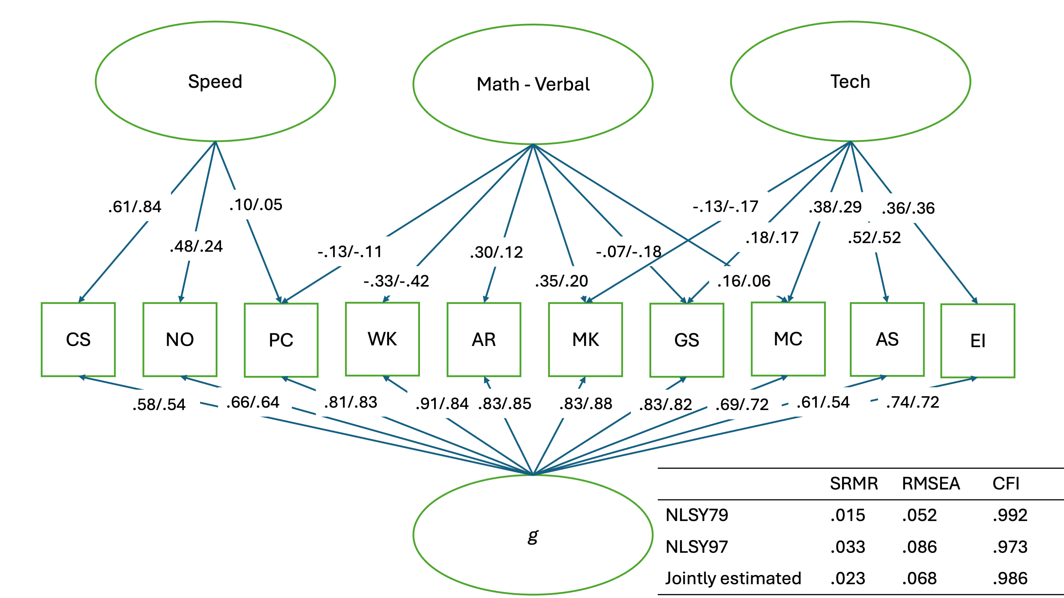
With confirmatory factor analysis, we tested the model implied by the NLSY79 EFA loadings in both NLSY samples. The results and fit statistics are shown in Figure 1. The model fit indices were very good in the NLSY79 sample, but only adequate in the NLSY97, even though the loadings were re-estimated within the sample. Another indicator of poorer fit in the NLSY97 was that to avoid negative residual variance for coding speed, we had to constrain it to be equal to zero. When the model was estimated jointly across the samples, fit statistics were still acceptable.
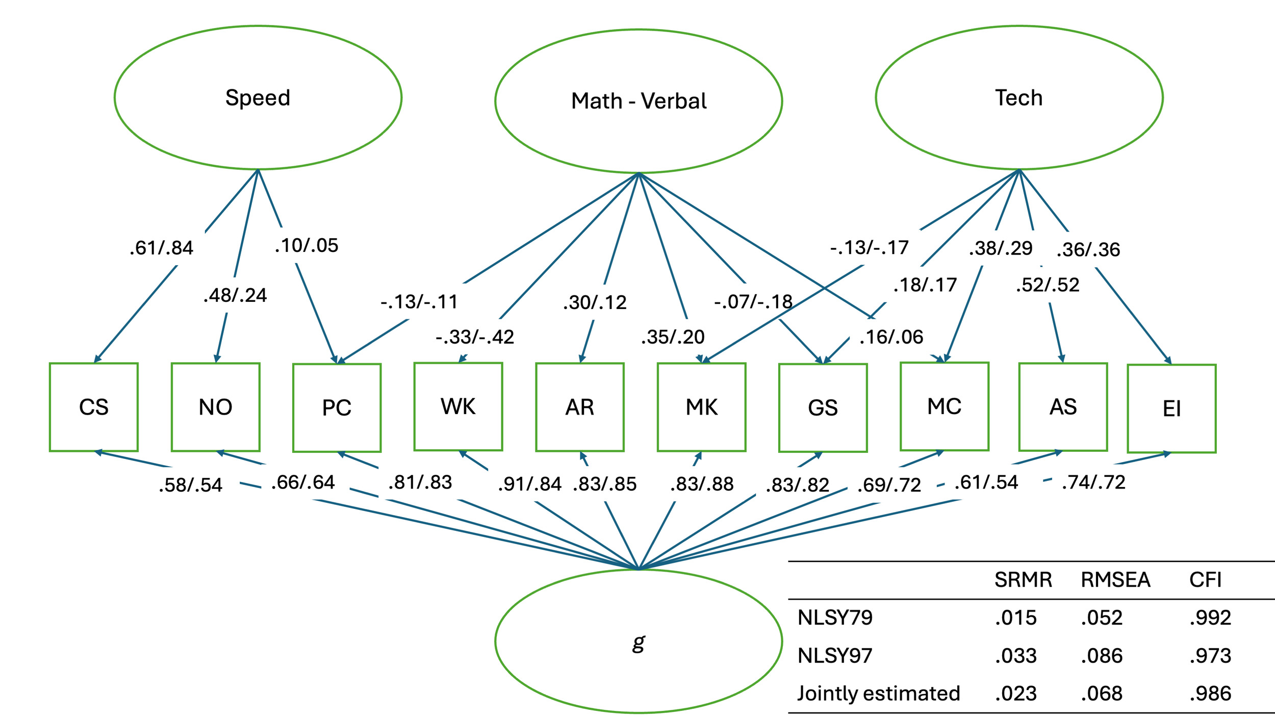
To examine metric invariance, we compared the model fit statistics before and after constraining the loadings to be equal. Changes in absolute fit indices indicated only a minor worsening of fit after the constraint In fact, when interpreting a fit statistic which penalizes model complexity, fit slightly improved We also performed the test with slight alterations, removing the constraint on coding speed residual variance in the NLSY97 and additionally imposing the same constraint in the NLSY79; in these cases, the changes in fit statistics after enforcing equal loadings became smaller.
While the global fit statistics were reassuring, there were specific loadings that changed dramatically across the NLSY samples. For example, on average the loadings on the speed factor changed by 0.17, and loadings on the math-verbal factor changed by 0.11. By contrast, the average loadings on g and tech changed by around 0.03. These large changes made us skeptical that the latent factors were capturing the same traits across samples. As a robustness check, we chose to repeat many of our main analyses using principal components instead of latent factors.
Tucker’s congruence coefficients (Tucker, 1951), which quantify the similarity of the factor loadings across samples, also supported our judgment that the math-verbal and speed factors were highly dissimilar across samples. In the confirmatory factor analysis, the coefficients were extremely high for g and tech By contrast, the coefficients for math-verbal and speed were of a magnitude considered between “fair” and “good” by experts Lorenzo-Seva and Berge (2006). Tucker coefficients, presented in Appendix Table A2, applied to the exploratory factor analyses provided a similar interpretation.
To assess the validity of our latent factors, we predicted a range of school examinations and of cognitive ability tests in Appendix Table A4. Across every math test, the math-verbal factor had a positive regression slope, and it had a negative slope on each verbal test. Curiously, in the NLSY97, the tech factor was a significant negative predictor of performance on math tests. Weaker loadings of the math ASVAB subtests on the math-verbal factor in NLSY97 may explain this result. The ratio of the effect of specific abilities to the effect of g was typically much smaller on IQ and the ACT than on the math and verbal tests. This gave us confidence that our latent factors really were capturing specific abilities rather than general intelligence, since IQ and the ACT would mostly reflect g.
In Appendix Table A5 we performed the same analysis, but using principal components instead of latent factors. PC1 had the largest regression slopes. The slopes of the other PCs were consistently more positive on the verbal tests than on the math tests, or vice versa, across the NLSY samples. Overall, the regressions suggested PC1 was a reasonable proxy for g, while the other PCs proxied mathematical and verbal abilities.
Predicting SES Measures
Table 2 shows the regressions of cognitive abilities on aspects of SES. The effect size of the specific abilities as a fraction of the effect size of the g ranged from 0.30 to 0.57. Consistently across the NLSY samples, the tech ability was negatively associated with education and occupational status, although it was unrelated to income. The effects of speed and math-verbal on the SES measures were inconsistent across samples. For example, in the NLSY79 math-verbal predicted education and occupational status, but in the NLSY97 it only predicted income. These inconsistencies implied that the effect of specific abilities may have changed between the two generations. On the other hand, the latent factors may have differed slightly across generations.
Appendix Table A6 shows the effects of the cognitive abilities stratified by sex. Tech had a less negative effect in men than in women for each dependent variable in each of the samples. For income, tech had a positive association in men in NLSY79; in NLSY97), but a negative association in women in NLSY79; in NLSY97). The importance of specific abilities for income was very high in men for both NLSY samples in NLSY79; in NLSY97). In the NLSY79, math-verbal had more positive effects in men than in women. Also in the NLSY79, speed had a larger effect on occupation status in women compared to men. General intelligence had larger effects on income in women as compared to men, which has been noticed before in the NLSY (Castex & Kogan Dechter, 2014; Lin et al., 2018).
To examine the sensitivity of our results to our methodology, we ran several robustness tests. When we used principal components, instead of latent factors, in Appendix Table A10, PCs two through four showed very different associations with income when compared across the NLSY samples. This result suggested that the changing effects of the specific abilities were not an artifact of our latent variable model. Nevertheless, the effects of the latent variables were still sensitive to modeling choices. In Appendix Table A7 we presented exploratory structural equation model (ESEM) estimates. In these models, all the subtests had non-zero loadings on each latent factor. In the NLSY79, the effects of speed on SES were much larger in the ESEM compared to the SEM in Table 2. In Appendix Table A8, we presented the results of a bifactor model created from a Schmid-Leiman transformation. In every robustness test, the relative importance of specific abilities was of similar size to estimates from our main specification.
There are further robustness tests we do not report in the manuscript: running the analysis using full-information maximum likelihood instead of maximum likelihood estimation, using sampling weights (for round one of the survey), and performing the models without pre-residualizing the ASVAB subtests on demographic variables. These changes had only trivial effects on the results, and raw output from the analyses can be found on OSF.
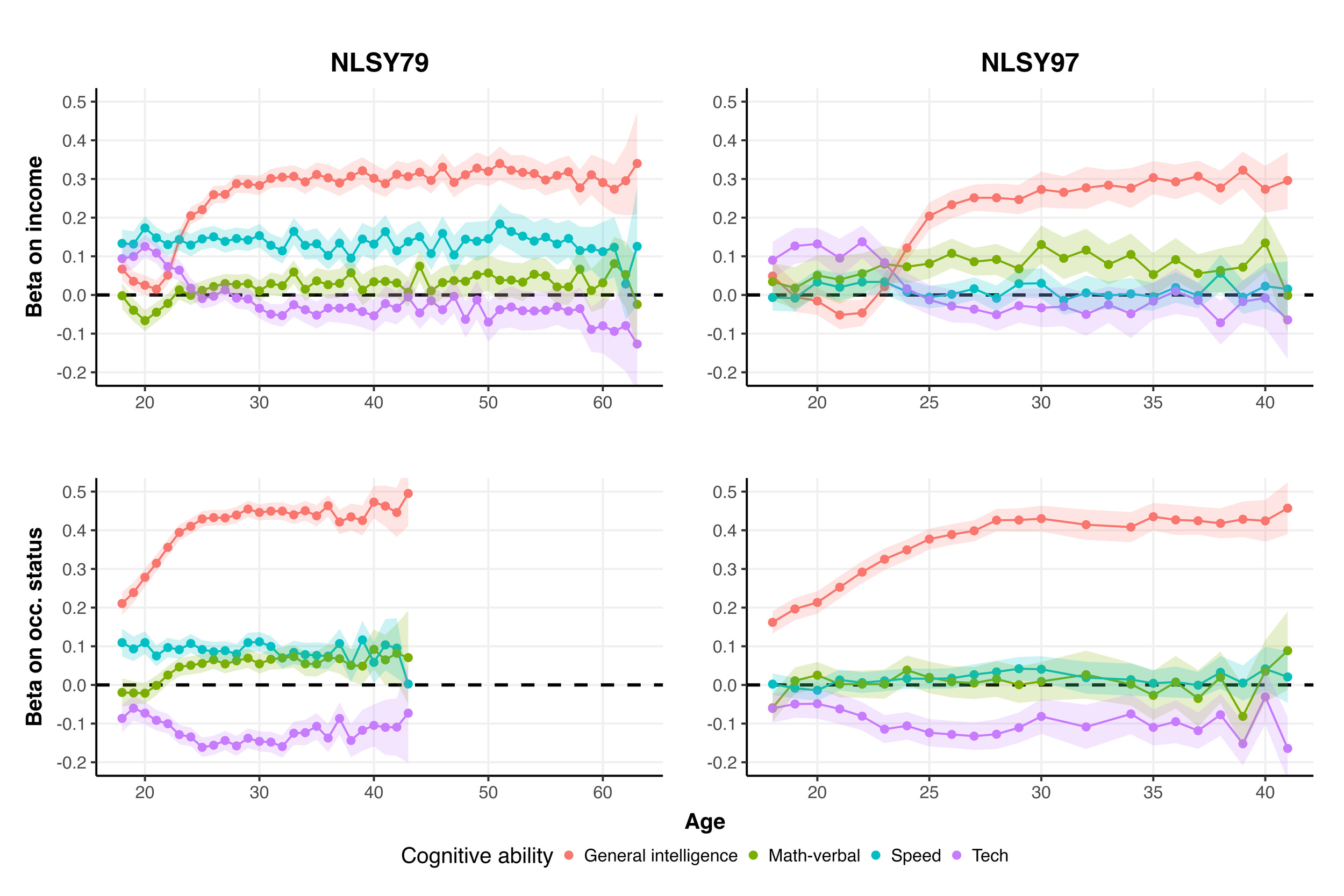
The association between cognitive abilities and SES was not constant over the lifespan. In Figure 2 we plot the effects of cognitive abilities at different ages. Before the age of 25, g’s effect on income was very small—negative even at ages 21 and 22 in the NLSY97. The effect of tech was reversed; it had positive effects on income during participants’ early 20s before becoming null or even negative later in life.
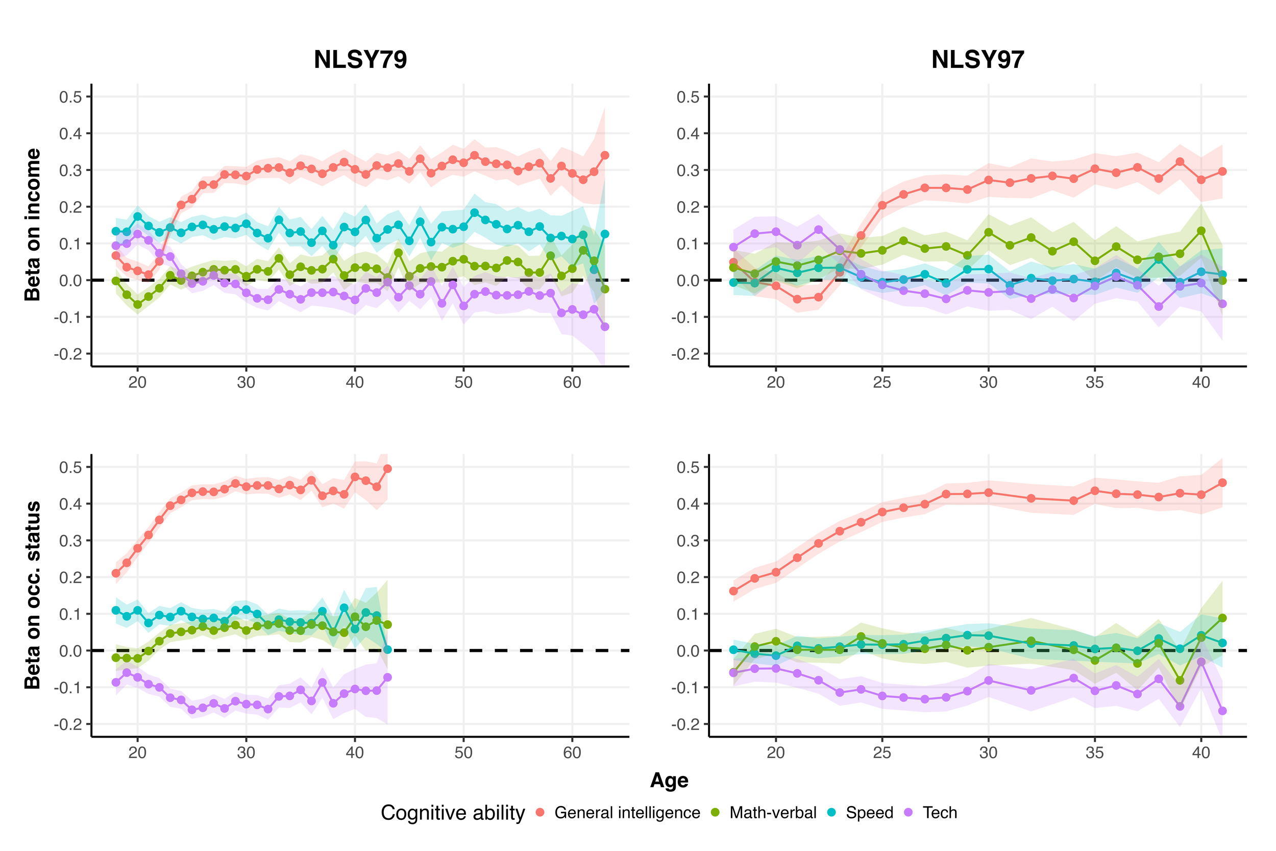
The effect of cognitive abilities on occupational status was relatively more stable. General intelligence always had a clearly positive effect on occupational status, albeit still increasing in the 20s. The tech factor had a negative association with occupational status, regardless of age, and did not change much. Exact values for the relative importance of specific abilities can be found in Appendix Table A9.
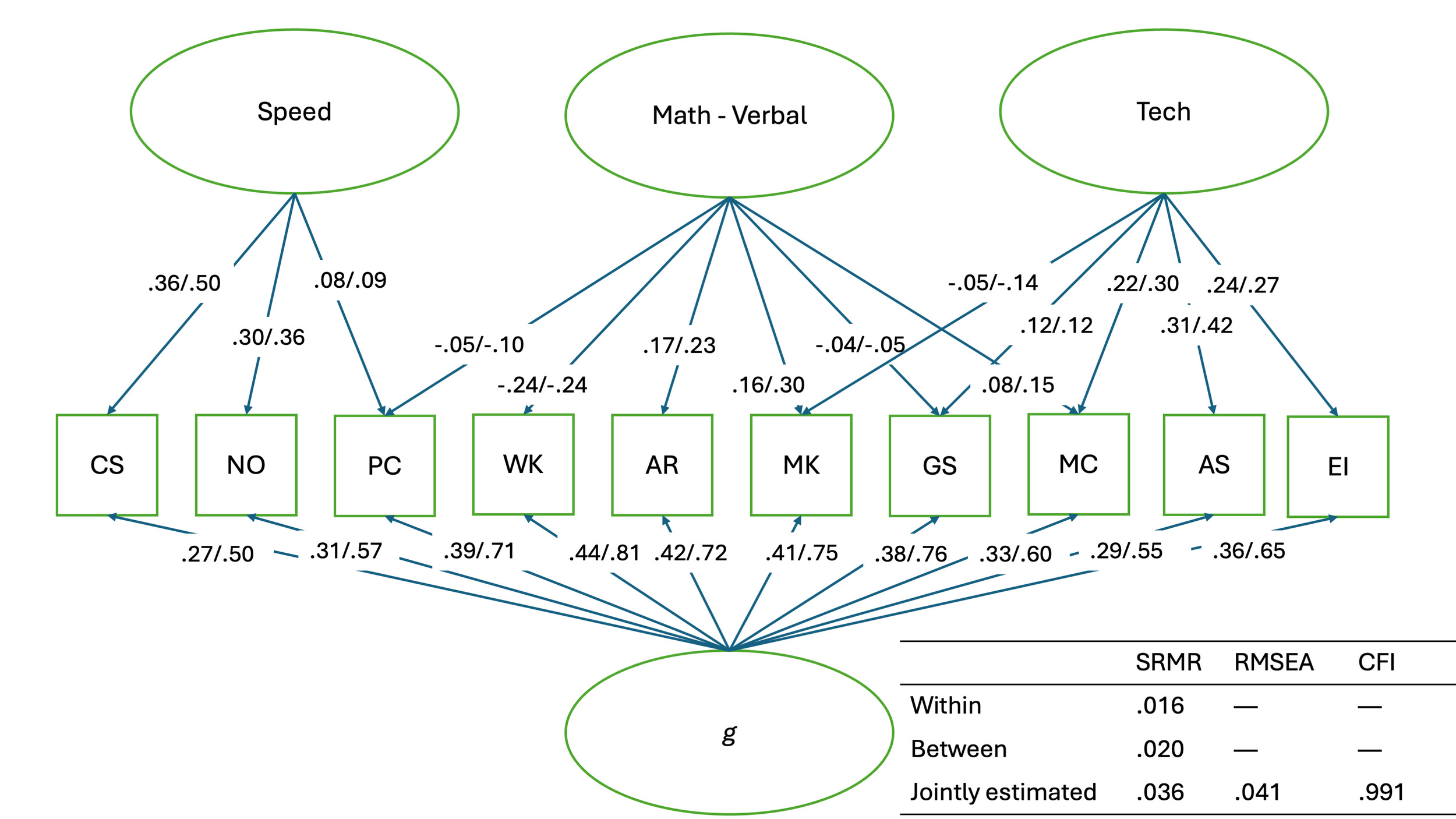
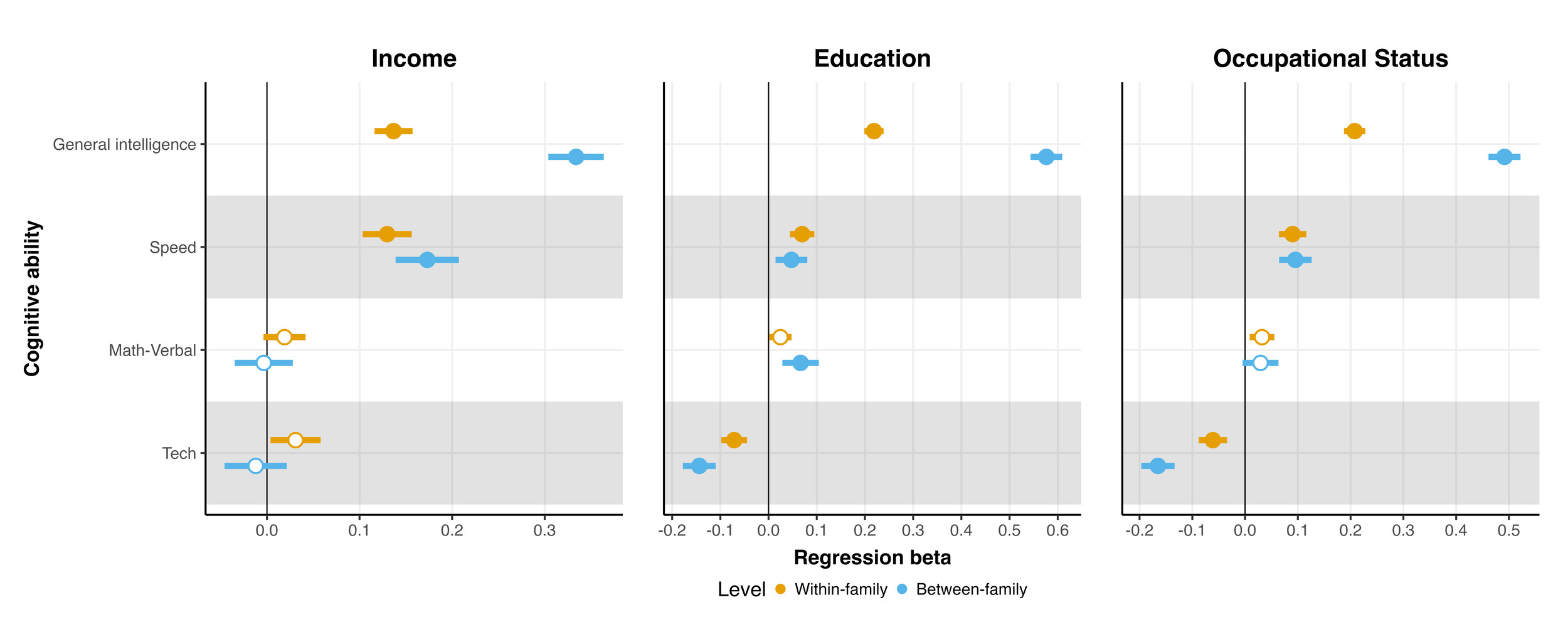
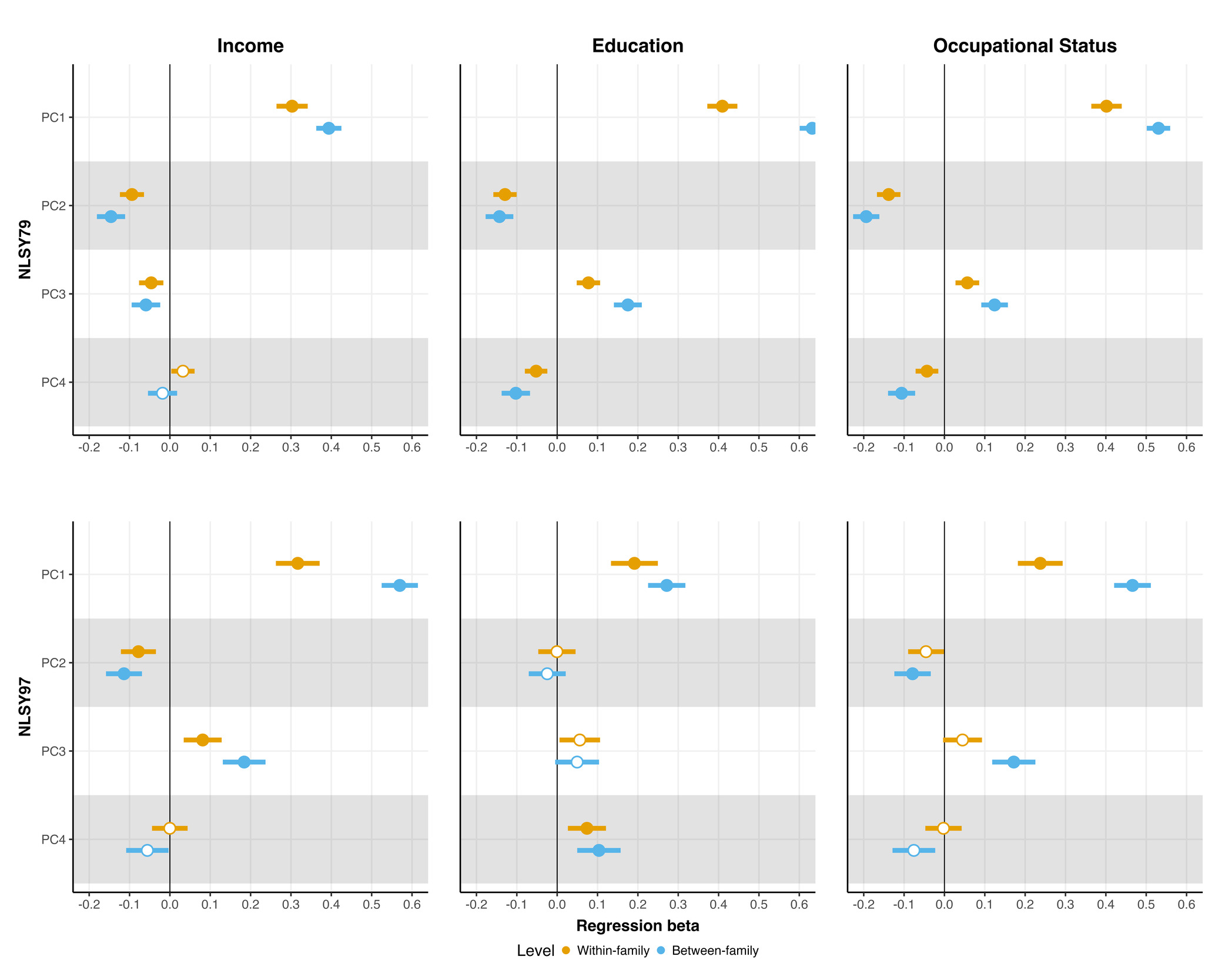
The effects of cognitive abilities might be confounded by family upbringing. To evaluate the issue, we decomposed the variance of the cognitive abilities into within-family and between-family factors. For the NLSY79, loadings of ASVAB tests on the latent factors are presented in Appendix Figure A1 and the factors’ associations with SES are presented in Figure 3. The model failed to converge in the NLSY97.
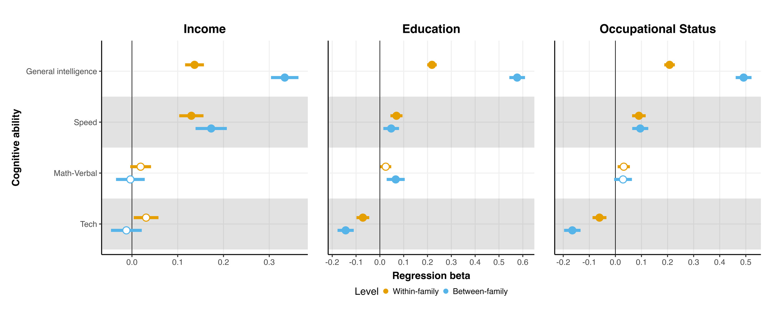
Each association observed in the full sample also appeared within families. With regard to general intelligence and the tech ability, the between-family effect sizes were often much larger than the within-family effect sizes. The regression slope of general intelligence was around twice as large for between-family variance as for within-family variance. By contrast, the effect sizes of the speed and math-verbal abilities were similar within and between families.
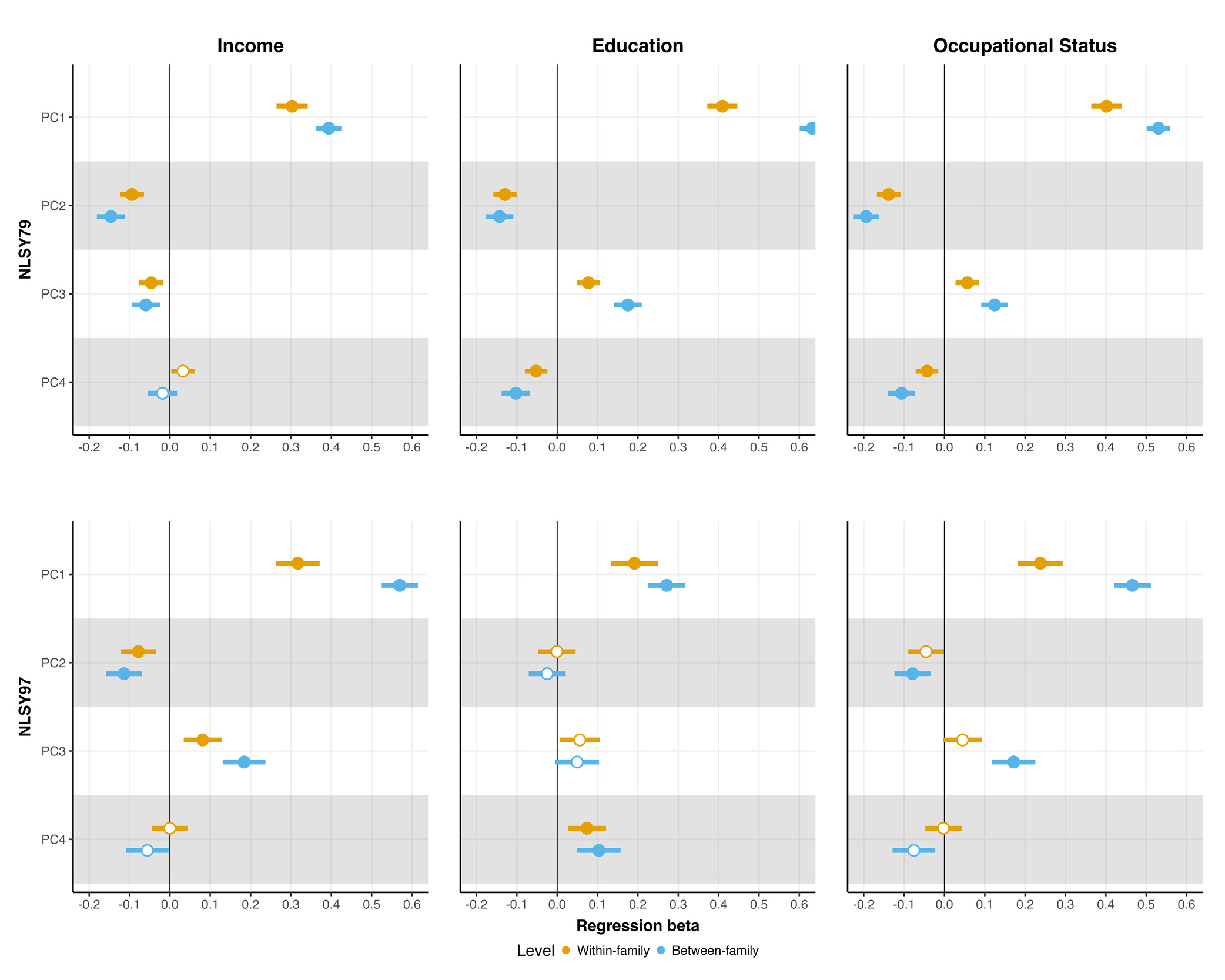
A difficulty with comparing the effects of within and between-family effect sizes is that the variance of cognitive abilities may not be the same within and between families. Latent variables, having no constant unit, cannot distinguish between the between-family effect being larger and its variance being larger. As a solution, we compared the effects of principal components within and between families in Appendix Figure A2.
When using principal components, the differences between within- and between-family effects were diminished, consistent with the between-family variance in cognitive abilities being larger than the within-family variance[1]. There was, however, a substantial difference in the effect of PC1 on education and occupational status. For example, in the NLSY79, the within-family effect on occupational status was and the between-family effect was This large a difference could not be explained by measurement error[2].
Occupational intelligence
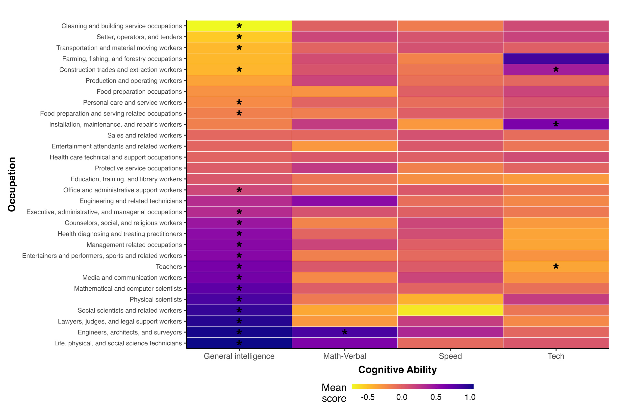
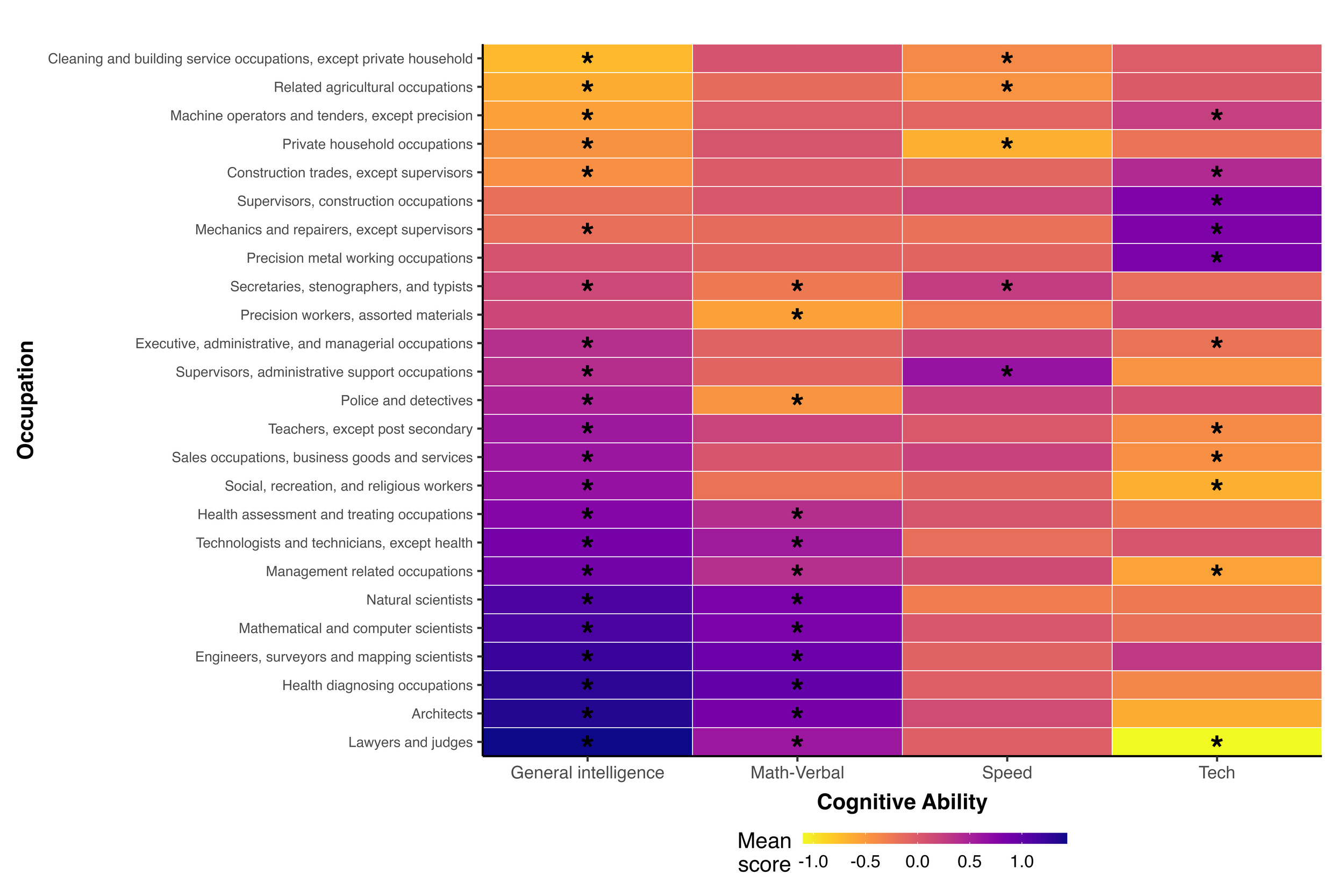
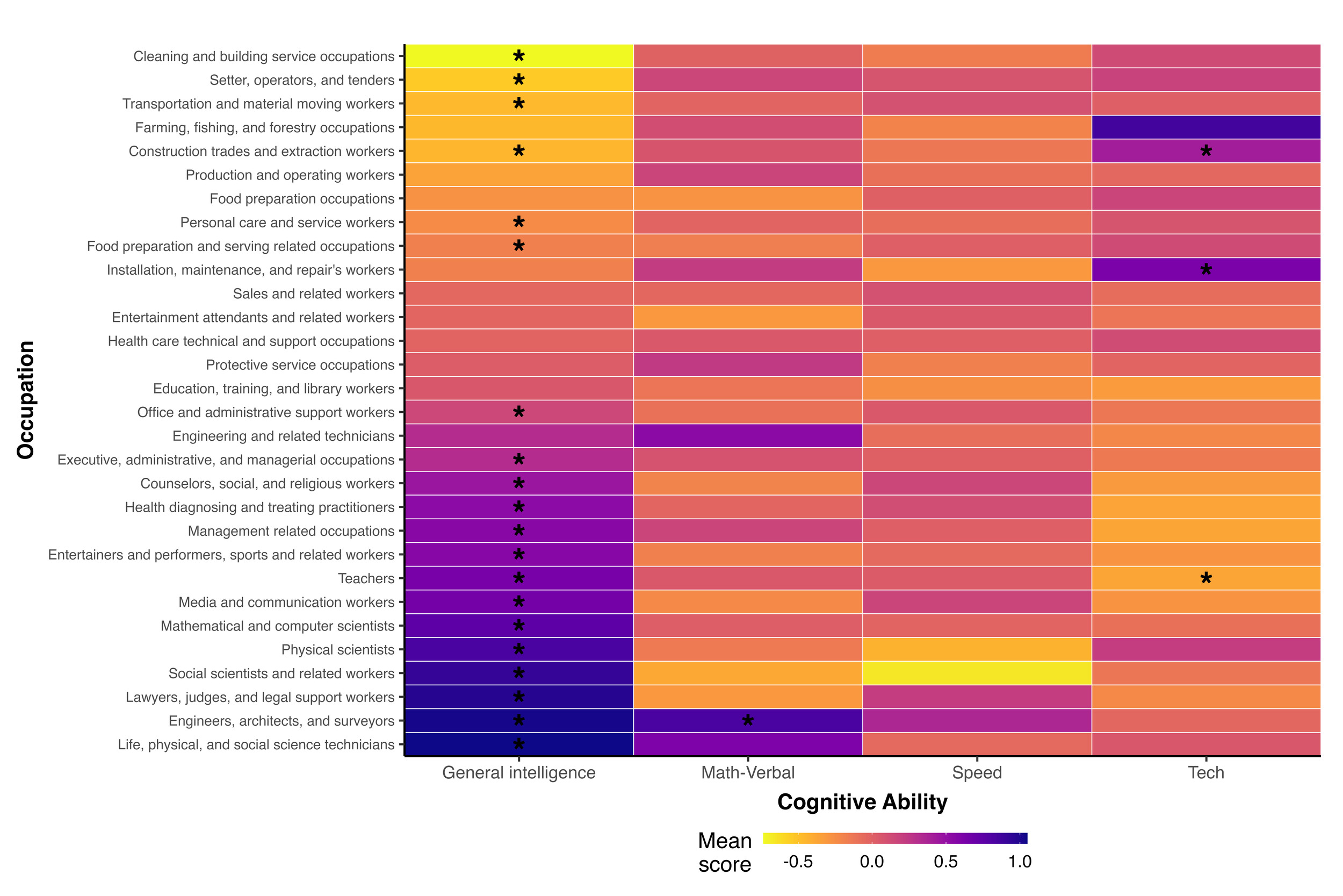
Estimates of the average cognitive ability of all occupations, and their standard errors, are given on the accompanying OSF page for this paper. In Figure 4, we present the average level of cognitive ability for a select group of 25 occupations from the 66 NLSY79 occupations with more than five occupants. These are jobs where the mean of at least one of the specific abilities is significantly different from zero
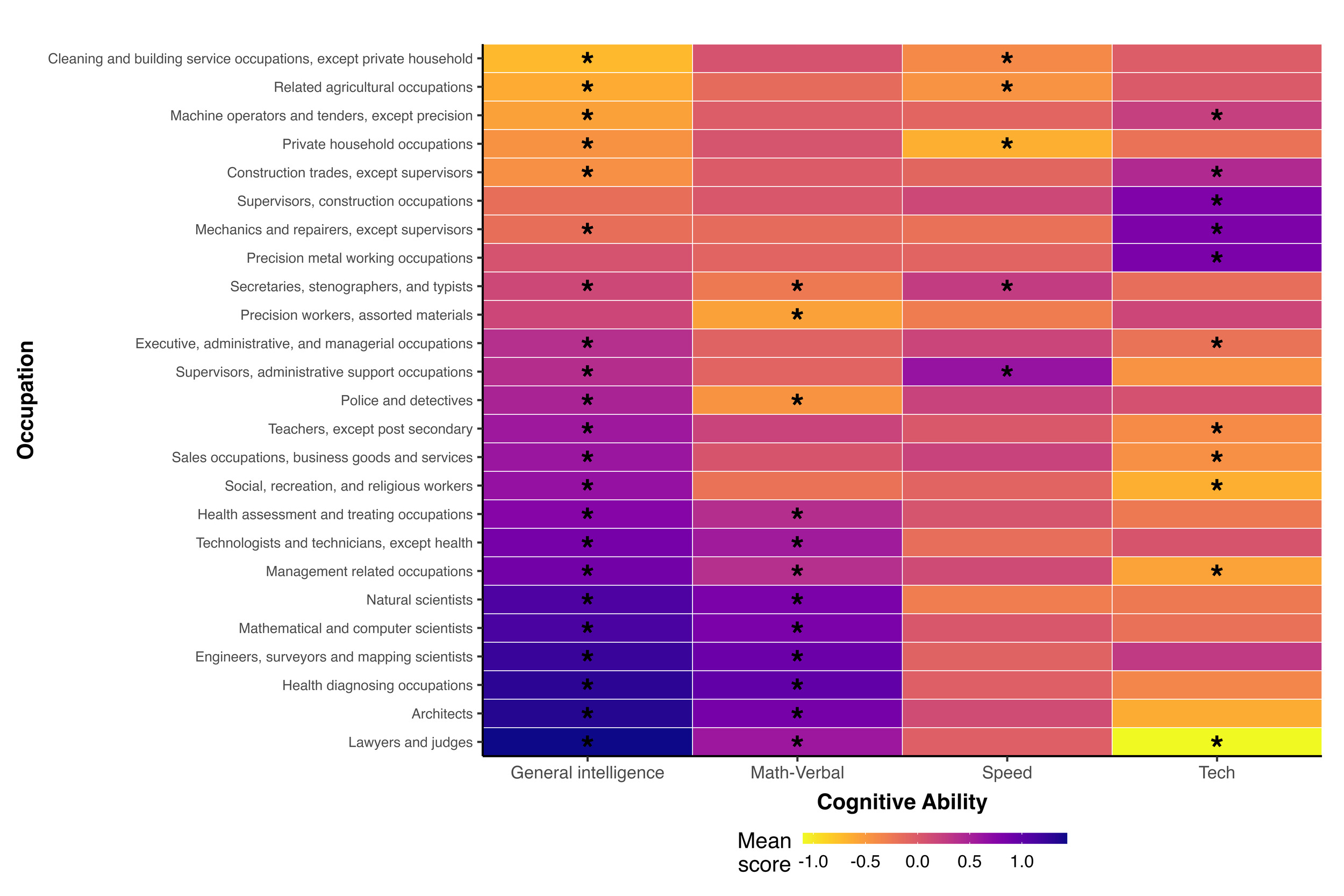
The rankings of general intelligence appeared intuitive, with cleaning occupations and machine operators (not including precision machines) having a low level of intelligence, while scientists, lawyers & judges and health diagnosing occupations (which include doctors) were among the most intelligent.
Two occupational categories had a significant positive average speed ability—Secretaries, stenographers, and typists and Supervisors, administrative support occupations, while three had a significant negative average speed ability—Cleaning and building service occupations (except private household), Private household occupations, and Related agricultural occupations. The broad name of related agricultural occupations specifically includes groundskeepers, animal caretakers, graders, and inspectors of agricultural products.
There were twelve occupations where math-verbal ability was significantly different from zero. The high math-verbal occupations included natural scientists, doctors (health assessment and treating occupations), engineers, and mathematical & computer scientists. The low math-verbal occupations included police, precision workers and secretaries, stenographers, and typists.
The high math-verbal occupations tended to also have higher general intelligence. For example, lawyers and judges had a very high math-verbal ability when stereotypes would suggest they should be better at verbal abilities than mathematical abilities. In fact, the average general intelligence of an occupation had a correlation with the average math-verbal ability of an occupation at This did not replicate in the NLSY97. See Appendix Table A11 for a correlation matrix of occupation average cognitive abilities in the NLSY79 and NLSY97. A possible explanation is that the math-verbal factor is partly capturing variation in general intelligence in the NLSY79, as might be expected from its positive regression slope on IQ in Appendix Table A4.
Eleven occupations showed a significant non-zero tech ability. High tech occupations included mechanics & repairers, construction workers, and precision metal workers. By contrast, lawyers & judges, management, sales workers, teachers, and social & religious workers had low tech abilities. General intelligence was negatively correlated with tech ability across occupations a pattern which also appeared in the NLSY97. There were some exceptions to this trend: engineers had high tech ability and high g while forestry and logging occupations had low tech ability and low g Nevertheless, the specific abilities of these exceptions were not significant after multiple correction
Because the NLSY97 had a smaller sample size and used broader occupational categories, only four groups showed a statistically significant deviation from zero in their group-factor abilities: engineers exhibited high math-verbal ability; teachers displayed low technical ability; construction trades and extraction workers demonstrated elevated technical ability; and installation, maintenance, and repair workers scored high on tech ability. These results were obviously congruent with the findings in the NLSY79.
A reviewer noted that the occupation results appeared to map onto the RIASEC taxonomy (Holland, 1959, 1973) of occupational interests. To examine this insight, we obtained RIASEC vocational interest scores for the occupations of participants and predicted them with our latent factors of cognitive ability in Appendix Table A12. General intelligence predicted occupations with lower realistic interests but higher values for all the other interests. Nevertheless, specific abilities also played a substantial role; ranged from 0.26–1.10. Tech ability predicted being in realistic occupations and avoiding the other categories, particularly social. Speed was positively associated with enterprising and conventional occupations, while being negatively associated with realistic occupations. In both NLSY samples, math-verbal was associated with investigative occupations, but in the NLSY97 it was negatively associated with social and enterprising occupations while also being positively associated with realistic occupations.
Occupational clustering
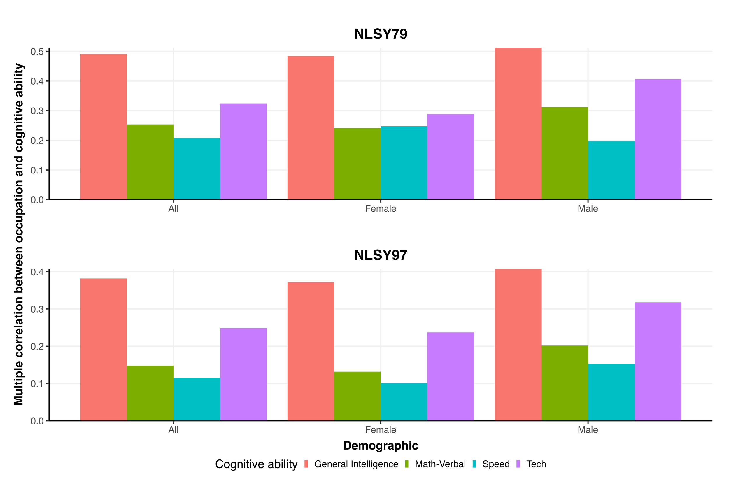
Figure 5 plots our metric of occupational clustering—the multiple correlations of occupation on each cognitive ability. Clustering was strongest for general intelligence, with a multiple correlation of .49 in the NLSY79. In other words, occupation explained 24% of the variance in general intelligence, which is very similar to previous estimates (Huang, 2013; Wolfram, 2023). All cognitive abilities showed weaker clustering in the NLSY97, presumably because there were half as many occupational categories in this sample.
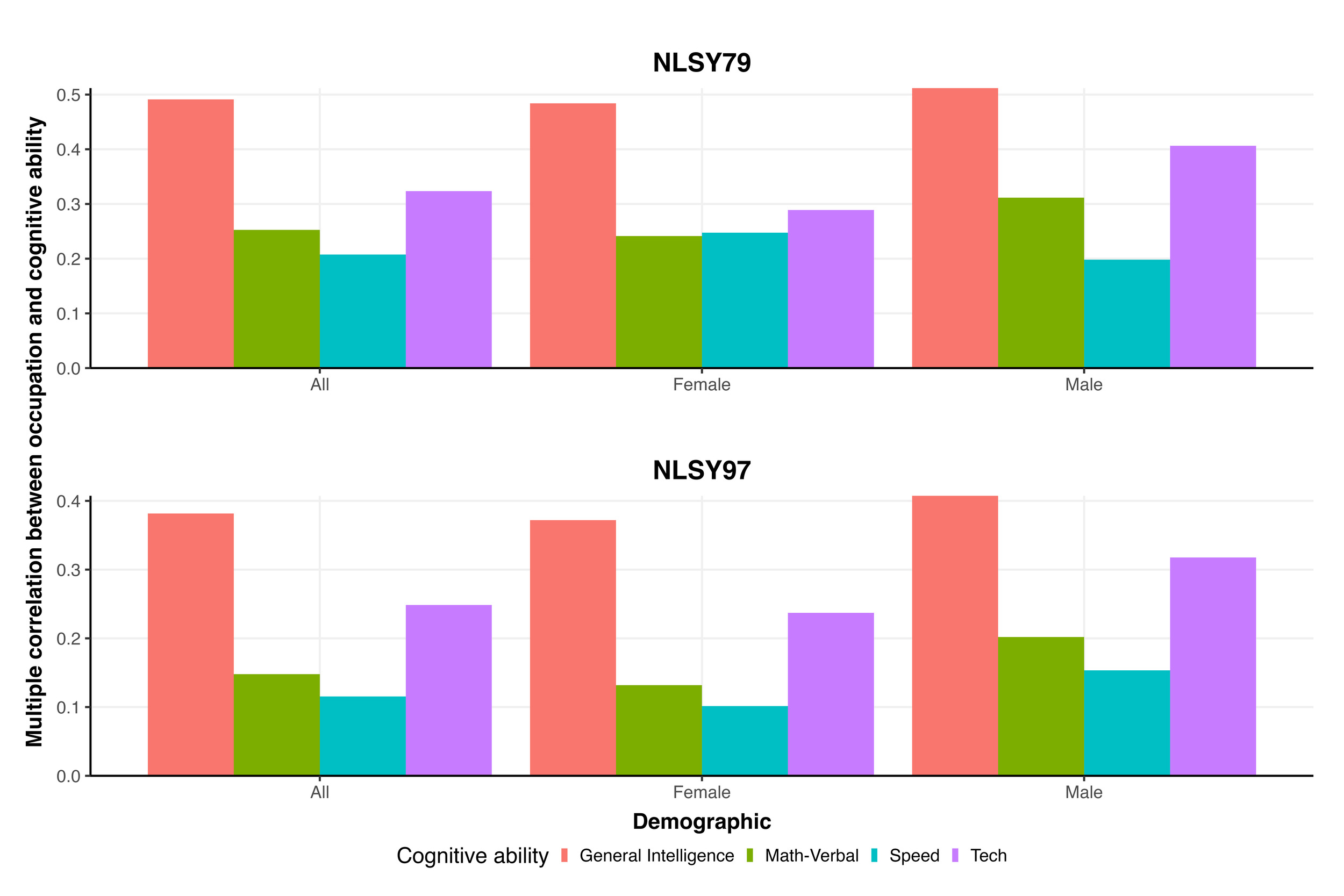
The second-highest amount of clustering was for tech ability, with a multiple correlation of .32 in the NLSY79 and .25 in the NLSY97. We calculated the degree of occupational clustering within each sex and found clustering on the tech factor to be substantially higher in men—the multiple correlation was .12 larger in the NLSY79 and .08 larger in the NLSY97.
The math-verbal and speed abilities also clustered by occupation, albeit less noticeably. The math-verbal factor showed much less clustering in the NLSY97. This ability might be less important in the later cohort. Alternatively, the latent factor may differ across cohorts, or it might be an artifact of the different occupational categories.
Discussion
Are specific abilities relevant to socioeconomic outcomes? Our answer is a clear yes. To be precise, we estimated that specific abilities are at least as important as general intelligence in predicting education, income, and social status.
The effects of the speed and math-verbal abilities were inconsistent across samples, indicating economic conditions may have changed or that the cognitive abilities captured were somewhat different across samples, a possibility we return to below. In contrast, the tech specific ability showed consistent negative associations across samples with educational attainment and occupational status. However, when stratified by sex, tech was associated with greater income in men and lower income in women.
The associations with tech ability accord with prior tilt research, which has shown that a spatial tilt predicts lower educational attainment and academic underachievement (Edwards et al., 2025; Gohm et al., 1998; Lakin & Wai, 2020). As originally proposed by Gohm, Humphreys, and Yao (1998), individuals with strong spatial ability may exhibit lower interest in academic curricula and instead prefer earlier labor market entry, particularly into blue-collar occupations aligned with their interests. Consistent with this interpretation, the tech factor loaded strongly on Mechanical Comprehension and vocational knowledge (e.g., Auto and Shop Information), domains that are more closely aligned with non-academic career pathways.
Many features of our analyses help clarify what causal relationships may exist between specific abilities and SES. Cognitive ability was measured in youth, before the age of 23, yet specific abilities were predictive of outcomes for many decades. This temporal ordering rules out reverse causation—adult SES cannot cause earlier ability variation.
We found that siblings who share the same biological parents but differ in specific abilities also tended to differ in SES. This suggests the relationship between specific abilities and SES cannot be entirely explained by confounds from upbringing. To our knowledge, we were the first to directly estimate and compare the effects of within-family and between-family variance in cognitive abilities on any outcome, let alone SES. Between-family variance was generally more important, but this was primarily because cognitive abilities differ more across families than within them. This pattern is expected if there is assortative mating for cognitive abilities or environmental influences on cognitive abilities that are shared between siblings. We did, however, find evidence that general intelligence has a larger effect on education and occupational status between families rather than within families.
The repeated surveying allowed us to estimate the relationship between specific abilities and SES at different points in life. General intelligence is known to become more important for SES with age before stabilizing in midlife (Ganzach, 2011). By contrast, we found different and telling patterns for other abilities. The effects of speed and math-verbal abilities appeared constant over time. The effect of tech ability on income was initially positive before turning negative after the mid-20s, but its effect on occupational status was always negative.
Apart from analyzing how specific abilities relate to overall SES, we also examined how they affect occupational choice. Average abilities in different occupations were consistent with stereotypes. For example, mechanics and metal workers were high in tech ability. Owing to a limited sample size, we could only identify occupations with unusual specific abilities. The sample size also prevented us from confidently analyzing the cognitive profiles of all the occupations in the NLSY.
The associations between cognitive abilities and occupations mapped onto the RIASEC vocational interest taxonomy: math-verbal was associated with investigative occupations, tech with realistic occupations, and speed with enterprising and conventional occupations. This partly replicates associations between cognitive abilities and individuals’ vocational interests (Ackerman & Heggestad, 1997; Pässler et al., 2015)—spatial ability is related to realistic interests. However, both mathematical and verbal abilities are related to investigative abilities, so it is not obvious that our factor representing relative performance between these two domains should predict investigative interests.
The degree of clustering by specific abilities was substantial. In the NLSY79, clustering by tech ability was 66% of the magnitude of clustering by g. Clustering by tech ability was substantially stronger in men than in women, implying men depend upon this ability more to guide their occupational choices. In men, clustering by tech was 79% as strong as clustering by g in the NLSY79.
The extent to which specific abilities have causal effects remains uncertain, despite the longitudinal and within-family analyses. Investment theory states that individuals put resources into developing specific cognitive abilities (Cattell, 1987, pp. 138–46). This investment is directed by interests. Someone interested in cars, for example, would spend time learning about cars and therefore perform better on the auto and shop information subtest of the ASVAB. Consistent with the view that specific abilities reflect interests is the fact that they predict college major (Coyle, 2018, 2019; Coyle et al., 2014; Humphreys et al., 1993; Shea et al., 2001). It is possible that it is these interests that are causing differences in SES, rather than their associated abilities. Alternatively, these interests might actually be driven by the abilities. A related complication arises from anticipating the future. An individual who expects a higher SES or a certain occupation might invest in specific abilities that are in some way complementary, perhaps because the relevant occupations are easier. Future research ought to further test for causal relationships between abilities, interests, occupations, and social status. This has obvious policy implications—the utility of investing in an ability is dependent upon its causal effects.
There are several limits to the generalizability of our results. The first issue is that the tech factor proved to be the most important specific ability for predicting SES outcomes. Standard intelligence tests do not include questions about electronics or car mechanics, so the importance of the specific abilities they assess might be lower. On the other hand, it is possible that traditional IQ tests capture more relevant specific abilities. Moreover, the tech factor may partly reflect cognitive abilities already captured by traditional intelligence tests, such as spatial ability.
A second limitation is that the structure of cognitive abilities might not be easily generalizable. We found the parameters of our measurement models and prediction models were substantially different between the NLSY79 and the NLSY97. This suggests the specific abilities captured by cognitive tests may not reflect a stable set of latent cognitive abilities or causes more generally. The issue might be that the structure of cognitive ability has changed by cohort, or it might reflect changes in the ASVAB. In the NLSY79, it was administered at ages 16–23, but in the NLSY97 it was administered at ages 12–16 using computerized adaptive testing. The cross-cohort changes in the prediction models might also reflect that the socioeconomic effects of specific abilities change over time.
We are not the first to run into these issues. Studies of the Flynn effect (the fact that IQ scores have risen over generations) have found that the factor structures of cognitive ability tests change over time (e.g., Wicherts et al., 2004). If specific abilities do not appear to be stable across samples, it will be very difficult to identify stable effects across studies.
Model misspecification is likely a key limitation of our work. Model misspecification means that true latent factors may differ from those we have specified; our regression betas will thus reflect the effects of a mix of the true latent factors of cognitive ability. A hint of misspecification comes from our math-verbal ability, in which high values implied higher performance on math tests and lower performance on verbal tests. There may not have been enough verbal and numerical subtests to identify these latent abilities separately. Alternatively, this factor might exist if there is a trade-off between investing in math and verbal abilities. For example, Giannelis et al. (2025) estimated a negative genetic correlation between quantitative (residualized on g) ability and reading skills.
While model misspecification will mix up the effects of the true specific abilities, it might have little impact on the combined effect of all the specific abilities relative to g. What would be a bigger problem is if the effects of our supposed-specific abilities were inflated by capturing the effects of general intelligence due to model misspecification. In the NLSY79, but not the NLSY97, math-verbal ability was estimated to be high in very intelligent occupations which rely more on words than numbers, such as lawyers and judges. This would suggest that math-verbal ability was partly capturing general intelligence. We expect this issue to be minor, since the specific abilities weakly predicted performance on other IQ tests in the NLSY79.
Since bifactor models have been criticized for overfitting the data (Bonifay et al., 2017; Markon, 2019; Reise et al., 2016), we wanted to be sure our key result—the importance of specific abilities—was not an artifact of our particular model choice. We applied two other factor models: a Schmid-Leiman model reduced overfitting by imposing proportionality constraints, and an exploratory structural equation model allowed a closer fit by not constraining any loadings to zero. Reducing or increasing the potential for overfitting in these respects did not substantially alter our conclusions.
As an alternative to our latent variable modeling, we also used principal components of ASVAB subtests. It has been common to treat the first principal component as an approximation of g and the rest of the PCs as representing combinations of specific abilities (Ree & Carretta, 2022). Regardless of whether we used principal components or our latent factor model, specific abilities showed a moderate importance relative to g. Our conclusion that specific abilities matter is not an artifact of our particular latent variable models.
Our finding that specific abilities have at least 30% of the importance of g in predicting SES might seem surprising considering the cliché from Ree and Earles (1991) that they reflect “not much more than g”. How do we resolve these two perspectives?
Ree and Earles (1991), in predicting job performance from the ASVAB, found that using 10 principal components instead of one increased from to —an apparently minor increase of But their result is quite similar to ours when reported with the same metric we used, the ratio of the correlations of specific abilities to that of g—
The ultimate disagreement between our conclusion and that of Ree and Earles (1991) is subjective—is a fifth or a third of the effect of g a trivial or reasonable effect? The combined effects of specific abilities on SES in our study correspond closely to the median effect size in differential psychology (Gignac & Szodorai, 2016). By contrast, the effect of specific abilities in Ree and Earles (1991) corresponds to the 25th percentile of effects It is reasonable to think specific abilities have a moderate association with socioeconomic outcomes.
Regardless of how we label the size of the effects, we encourage much more research on specific abilities. By comparison, there are up to fourteen meta-analyses relating SES to measures of cognitive ability (Korous et al., 2022). If specific abilities have at least a third of the importance of general intelligence for socioeconomic status, then it would make sense for a third of all research to cover specific abilities as well as general intelligence.
Additional materials
Code, further descriptive statistics, raw results, and other materials are available on this study’s OSF page.
Acknowledgments
We would like to thank the anonymous reviewers for their helpful and insightful comments.
Declaration of Conflicting Interests
The authors declare no conflicts of interest.
Funding
The authors received no specific funding for this work.