

Introduction
The greatest advance in a century of behavioral genetic research has been the ability to predict individual differences in behavior directly from DNA in addition to estimating genetic effects indirectly using twin and adoption designs. After a disappointing decade of candidate-gene results that failed to replicate (Border et al., 2019; Chabris et al., 2012), by 2005, DNA microarrays made it possible to investigate hundreds of thousands of DNA variants (single-nucleotide polymorphisms, SNPs) in genome-wide association (GWA) analyses. In 2007, genome-wide association was shown to yield replicable associations with common disorders (The Wellcome Trust Case Control Consortium, 2007). However, the largest effect sizes of SNPs were extremely small, which led to the construction of polygenic scores (PGS) that aggregate SNP associations in a composite that can be used to predict individual differences in behavior (Purcell et al., 2009). Currently, the strongest PGS predictions in the behavioral domain can be made for cognitive and educational traits, which include intelligence, cognitive abilities, educational achievement, and years of schooling (educational attainment). PGS can predict, in independent samples of unrelated individuals, up to 11% of the variance for cognitive abilities (Procopio et al., 2024), 18% for educational achievement (Allegrini et al., 2020), and 14% for educational attainment (Okbay et al., 2022).
It is not coincidental that cognitive and educational traits not only show the strongest PGS prediction, but they also show the greatest evidence of family-level (between-family, BF) effects such as population stratification, assortative mating, and passive genotype-environment correlation that are not reflected within families (WF), as illustrated in Figure 1. One of the most important goals of PGS is to predict individual differences in the population; for example, predicting which children are likely to have problems learning to read. For this reason, estimates of the variance explained by a PGS are based on unrelated individuals, that is, one individual per family. In contrast, the WF contribution to this population prediction can be assessed by regressing sibling PGS differences with sibling trait differences. WF differences arise largely from variations in the meiotic inheritance of alleles, a process that is essentially random. This approach excludes BF effects, as siblings share the same parents and, consequently, the same family-level genetic influences from assortative mating, population stratification, and passive genotype-environment correlation (Benyamin et al., 2009). These BF effects can therefore be indexed as the extent to which the population correlation exceeds the WF correlation.

Although predicting individual differences between unrelated individuals in the population capitalizes on both WF and BF genetic effects, the partition of the PGS population prediction into its WF and BF components can be useful. For example, predicting sibling differences in a trait from their PGS differences is restricted to WF effects (Howe et al., 2022) and BF effects point to family-level sources of genetic variance, including assortative mating, population stratification, and passive genotype-environment correlation.
BF effects have been found most often in the cognitive domain. For example, an early report (Selzam et al., 2019) from the dataset used in the present study found substantial BF effects for cognitive abilities and educational achievement but not for non-cognitive traits (anthropometric, personality, and health). Other studies have also reported BF effects on cognitive abilities (Howe et al., 2022; Lello et al., 2020), educational achievement (Howe et al., 2022; Malanchini et al., 2024; Zhou et al., 2024), and educational attainment (Belsky et al., 2018; Howe et al., 2022; Okbay et al., 2022; Willoughby et al., 2021).
Sibling pairs provide a straightforward analysis of within- and between-family effects because of random segregation of alleles during meiosis and because they grow up in the same family. However, parents and offspring can also help distinguish individual-level genetic effects from family-level effects, although parent-offspring comparison rests on modeling assumptions about Mendelian transmission and partially random mating (Guan et al., 2025; Kong et al., 2018). In contrast, a within-sibship comparison, though less powerful statistically due to reduced sampling variation from sibling differences, provides a robust benchmark with minimal assumptions. It is also less susceptible to the genetic effects arising from population stratification and assortative mating. More specifically, the present study focused on dizygotic twins, a special type of sibling who are exactly the same age, which maximizes the power of within-sibship comparisons by controlling for age effects.
It should be noted that this issue of WF and BF effects is different from another topic of current interest, environmentally mediated genetic effects, often referred to as genetic nurture (Bates et al., 2018; Belsky et al., 2018; Cheesman et al., 2020; de Zeeuw et al., 2020; Demange et al., 2022; Eilertsen et al., 2021; Kong et al., 2018; Nivard et al., 2024; Su et al., 2022; Tan et al., 2024; Tanksley et al., 2024; van der Laan et al., 2023; Wang et al., 2021; Willoughby et al., 2021). Genetic nurture is deduced when parental PGS, independent of offspring PGS, predicts the offspring trait, suggesting genetically indexed environmental transmission. Genetic nurture is a BF effect related to passive genotype-environment correlation, but it is a complicated issue involving genetic associations with shared environmental influence, which we address in another paper (Plomin et al., 2024).
The Present Study
Selzam et al. (2019) reported results for intelligence at age 12 and for educational achievement at age 16. Here, using 3306 dizygotic twin pairs, we systematically investigate WF and BF effects developmentally at six ages (7, 9, 10, 12, 16, and 25) for verbal and nonverbal abilities as well as intelligence and educational achievement, with additional assessments of high school and university grades at ages 18 and 22 and, in adulthood, for educational attainment. Twin heritability estimates for intelligence increase developmentally (Haworth et al., 2010) and there is some evidence that PGS prediction of intelligence and educational achievement also increase developmentally (Allegrini et al., 2019; Selzam et al., 2017). However, we are not aware of previous studies that investigated cognitive and educational developmental changes in WF and BF contributions to the population PGS prediction.
The present study also attempted to replicate the finding from Selzam et al. (2019) that BF effects are mediated by SES in adolescence and to ask whether similar mediation is found in childhood and early adulthood. We also investigated whether WF and BF effects differ at the extremes of the distribution or for females and males. Analytically, we compared the results of the model used by Selzam et al. (2019) to a simpler model that just uses differences within pairs of DZ twins to estimate WF effects. We also included height and body mass index (BMI) from childhood to adulthood as negative controls, because their population genetic effects appear to be due almost entirely to WF genetic effects (Howe et al., 2022).
Materials and Methods
Sample
We drew participants from the longitudinal twin cohort study TEDS, which recruited 13,759 families with twins born between 1994 and 1996 in England and Wales (Lockhart et al., 2023; Rimfeld et al., 2019). Genotypic data was available for 10,346 TEDS participants. DNA sample collection and genotyping procedures are detailed in the Appendix A, with more information in our previous publication (Selzam et al., 2018) and the TEDS online data dictionary (https://www.teds.ac.uk/datadictionary/home.htm). Both the overall TEDS cohort and the genotyped subsample are representative of the UK population for their birth cohort. Data collection details were. Ethical approval was obtained from King’s College London Research Ethics Committee (References: PNM/09/10–104 and HR/DP-20/2122060). Informed consent was obtained before each wave of data collection.
The present study included 6972 unrelated individuals and 3306 DZ twin pairs assessed across three developmental periods: childhood (7, 9, and 10 years), adolescence (12, 14, and 16 years), and adulthood (18, 21, 22, 25, and 26 years). Unrelated participants were used for population genetic estimates and DZ twin pairs for within-family estimates.
Measures
In this section, we briefly describe phenotypic and genomic measures. Details are available in the Appendix B for the assessment of cognitive abilities and educational achievement at each age and for educational attainment in adulthood and the Appendix C for the construction of polygenic scores. We focused on five polygenic score predictors: intelligence (IQ3) (Savage et al., 2018), educational attainment (EA4) (Okbay et al., 2022), childhood BMI (Vogelezang et al., 2020), adulthood BMI, and height (Yengo et al., 2022). Notably, our participants were included in the original IQ3 GWAS. To avoid sample overlap, we did not use the publicly available summary statistics; instead, we obtained a special version of the summary statistics from the authors with the TEDS participants excluded, which we used for polygenic score construction. We used a combination of LDpred1 and LDpred2 in constructing the polygenic scores (Privé et al., 2021; Vilhjálmsson et al., 2015). These Bayesian approaches account for linkage disequilibrium (LD) by adjusting GWAS summary statistics based on an LD reference panel, allowing SNP effect sizes to be reweighted according to their correlations with nearby variants. LDpred retains all SNPs in the summary statistics, rather than discarding those in high LD regions, and assigns weights accordingly for use in polygenic scoring. Compared to Selzam et al. (2019), we approximately doubled the number of SNPs included in our genotypic sample (~1 million vs. ~515,000), enhancing the overlap with GWAS summary statistics and thereby improving predictive accuracy. In addition, we used updated GWAS summary statistics to reflect the most recent GWAS results available.
The IQ3 polygenic score was used to predict intelligence and cognitive abilities, including general cognitive ability (g) and its verbal and nonverbal components from childhood to early adulthood (ages 7, 9, 10, 12, 16, and 25). The EA4 PGS was used to predict our educational achievement and attainment outcomes (ages 7, 9, 10, 12, 16, 18, 21, and 26). We also included two anthropometric outcomes as negative controls. Height at all ages (7, 12, 14, 16, 22, 26) was predicted using the height PGS. We predicted BMI at age 7 using a childhood BMI PGS as the GWAS covered participants from 2 to 10 years old, while the rest of the ages (12, 14, 16, 22, and 26) were predicted using the BMI PGS from a BMI GWAS of adults.
Descriptive statistics for all measures are in Table G1.
Phenotypic Measures
General cognitive ability (g) and its verbal and nonverbal components were assessed at six ages: 7.15 (standard deviation = 0.26), 9.01 (0.28), and 10.07 (0.29) during childhood; 11.86 (0.61) and 16.48 (0.27) during adolescence; and 24.80 (0.86) in adulthood. Across these ages, our study had on average 2183, 2280, and 2256 unrelated participants for g, verbal g, and nonverbal g respectively, as well as 1032, 1078, and 1069 full DZ twin pairs. At each age, verbal and nonverbal abilities were assessed with intelligence tests, with g derived from the mean scores. At age 12, g was measured independently using a separate set of tests.
Educational achievement was measured at seven ages: 7.20 (0.28), 9.03 (0.29), 10.10 (0.29), and 11.53 (0.66) during primary school and secondary school; 16.31 (0.28) for the General Certificate of Secondary Education (GCSE) exams; 18.32 (0.30) for A-level; and 22.26 (0.92) for university grades. In the UK, A-levels are a two-year school option offered after completing compulsory education at age 16. The average sample size is 3079 unrelated participants and 1494 full DZ twin pairs.
Educational attainment was measured twice at ages 22.26 (0.92) and 26.42 (0.92), with its two precursors for enrollment in A-level exams and enrollment for higher education both measured at 18.32 (0.30). In the UK, A-levels are required for university entry. After applying for universities, enrolment in the university is required for completing higher education. The sample size is an average of 4463 unrelated participants and 2192 full DZ twin pairs.
Body Mass Index (BMI) and height were assessed at six ages: 7.11 (0.27) in childhood; 11.56 (0.69), 14.07 (0.58), and 16.48 (0.27) in adolescence; and 22.26 (0.92) and 26.42 (0.92) in adulthood. We had an average of 2804 and 2839 unrelated participants for BMI and height respectively, with 1374 and 1390 full DZ twin pairs. In childhood and adolescence, parents reported twins’ weight (in kilograms) and height (in centimeters). In adulthood, twins reported their weight and height. BMI was calculated later by researchers as kilograms per square meter.
Family SES was measured at birth, ages 7, 16, and 21. The composites were z-standardized and derived from mother and father employment categories coded using the standard occupational classification (SOC, https://www.ons.gov.uk/methodology/classificationsandstandards/standardoccupationalclassificationsoc/), mother and father highest level of educational qualifications, and household income.
Statistical Analyses
We have pre-registered the present study (www.osf.io/pg9w6). There are several deviations from the pre-registration. First, we narrowed the scope to cognitive and educational traits, reserving psychopathology traits for a subsequent paper. Second, we limited our statistical approach to within-sibship analyses, deferring parent-offspring analyses to another follow-up paper. Third, we excluded twin and multi-PGS analyses due to our refined focus. These adjustments were planned and implemented before carrying out any data analyses. Additionally, some of our current data were used in a cross-country collaborative study on educational achievement (Starr et al., in preparation).
Data Preparation
All analyses were performed using RStudio 2023.09.1 and codes are available on GitHub (https://github.com/YujingLinn/WFBF_CogEduAnthro). We first assessed potential effects of age, sex, birth order, zygosity, and sex-zygosity on our phenotypes (Table G2). We did not detect birth order or sex-zygosity effects, allowing us to randomly select one twin from each pair for population genetic analyses while retaining both same-sex and opposite-sex DZ twins for within-family analyses to increase power.
Significant mean age, sex, and zygosity effects were detected. To control for these effects, we employed two complementary approaches: 1) covariate-adjusted analyses—covariates were pre-adjusted for the phenotypes or added to the analyses; 2) covariate-stratified sensitivity analyses—phenotypes were stratified by covariates. We pre-adjusted our continuous phenotypes for age instead of adding it to the regression models, because age is a continuous measure and not relevant for the PGS. We also pre-adjusted the continuous phenotypes for sex, because PGS were derived from sex-adjusted GWAS, making them orthogonal to sex. However, for dichotomous phenotypes (i.e., A-level and university enrollment), we included age and sex in the main regression models to retain the binary values of zero and one.
Zygosity effects were relevant only at the population level, as the within-family analyses exclusively involved DZ twins. We conducted a zygosity-stratified sensitivity analysis and did not detect significant differences between MZ and DZ twins (Figure F1). Therefore, we did not further adjust our phenotypes for zygosity.
Additionally, to ameliorate ancestral and genotyping batch effects, the first ten principal components and genotyping chip were included as covariates for all main analyses.
Twin Pairwise Composite Construction
We calculated the phenotypic twin pairwise composites (i.e., differences, sums, means, and deviations from pairwise means) using the phenotypic data without adjusting for age or sex. Twins are matched for age. Sex adjustments were applied to the composite directly. We adjusted the twin pairwise means and sums using a three-level sex variable (i.e., same-sex female, same-sex male, and opposite-sex). For twin pairwise differences and deviations, we used a four-level sex variable (i.e., same-sex female, same-sex male, opposite-sex male, and opposite-sex female).
Sex-stratified sensitivity analyses were later performed on sex-unadjusted phenotypic twin pairwise composites to validate findings.
For the two dichotomous phenotypes of A-level enrollment and university enrollment, the twin pair composites were treated as three-level ordinal factors (e.g., both twins enrolled in A-level, only one twin enrolled, and no twin enrolled).
Genetic Effects
We used regression models to estimate population and within-family genetic effects. We first predicted cognitive, educational, and anthropometric traits from their corresponding PGS at the population level, that is, for unrelated individuals (i.e., one twin randomly selected per pair) across three developmental periods: childhood (7, 9, and 10 years), adolescence (12, 14, and 16 years), and adulthood (18, 21, 22, 25, and 26 years). The regression model was formulated as follows:
Yij=a0 +βPOP⋅PGSij+γ⊤Zij+εij
where i represents individual DZ twins (i= {1, 2}) in each family j. represents potential covariates, including sex, age, the first ten principal components, genotyping chip, and socio-economic status (SES). Additionally, is the intercept and is the error term. Age and observed sex were included as covariates in all analyses—as adjustment variables for continuous phenotypes and as covariates in regression models for dichotomous phenotypes. All continuous variables (predictors, outcomes, and covariates) were standardized to enable cross-regression comparison. Binary and three-level ordinal variables, including genotyping chip and sex, remained unchanged.
Multiple linear regressions (‘lm’ function from the stats package) were used for continuous phenotypes, while logistic regressions (‘glm’ function) were applied to dichotomous phenotypes. To aid comparability across models, logistic regression coefficients were converted to Pearson’s r using the transformation as follows (Chinn, 2000):
βtransformed=βoriginal√βoriginal2+π23
Additionally, we computed variance explained estimates as a complementary effect size metric. For continuous outcomes, we reported R2 from linear models. For binary outcomes, we calculated pseudo-R2 using the maximum likelihood estimator (‘pR2’ function, pscl package). Pseudo-R2 compares log-likelihood of the fitted model against an intercept-only null model (i.e., without predictors). This produces a 0-to-1 scaled measure of improved model fit, analogous to R2 in linear regression.
Percentile bootstrapping with 1000 iterations was performed to generate 95% confidence intervals and standard errors. Similar estimates were obtained across different ages within each developmental period and were aggregated using a random-effects model (‘rma’ function from the ‘metafor’ package) with restricted maximum likelihood estimation. Inverse variance weighting provided more precise estimates in the pooled results. This random-effects approach was selected to address heterogeneity between age groups, particularly given the differences in measurement tools across different ages. While some dependence between estimates may exist due to overlapping participants across waves, inverse-variance weighting remains a widely accepted and appropriate method in such cases—especially when individual-level multivariate modeling is not feasible or would substantially complicate interpretation. Our bootstrapped standard errors also help capture sampling variability.
Subsequently, we decomposed the total PGS prediction in the population into within-family and between-family components. For WF effects, we regressed pairwise differences in PGS on pairwise differences in the phenotype within full DZ twin pairs (Carlin et al., 2005; Lello et al., 2020):
(Yi1 − Yi2)= a0 + βWF(PGSi1−PGSi2)+γ⊤Zij+εij
where i1 and i2 denote individual twins in random orders from same-sex and opposite-sex DZ pairs, as birth order or sex-zygosity effects were not found for the phenotypes. A four-level sex dummy covariate (i.e., same-sex female, same-sex male, opposite-sex male, and opposite-sex female) was included to account for directional phenotypic differences in DZ pairs.
We used the ordered logistic regression (‘polr’ function, MASS package) to handle the three possible levels of pair differences for dichotomous outcomes. Estimates were transformed to Pearson’s r using Eq. 2. Pseudo-R2 was computed using the same method as the population predictions. We generated 95% confidence intervals using percentile bootstrapping (1000 iterations) and aggregated estimates within developmental periods using random-effects models with inverse variance weighting.
Then, following our operational definition, BF effects are quantified as the differences between the population and within-family predictions. To empirically assess the presence of BF effects, we subtracted WF from population predictions across 1000 bootstrap samples for each phenotype. We estimated the mean difference, 95% percentile-based confidence intervals (CIs), and a z-score derived from the bootstrap distribution (mean difference divided by its standard error) (Selzam et al., 2019). Statistical significance was assessed via a two-tailed z-test, with p-values further corrected for multiple comparisons using false discovery rate (FDR) adjustment.
Additional analyses are detailed in the Appendices D and E. In Appendix D, we applied a mixed-effects model to compare to the analyses described above (Carlin et al., 2005; Laird & Ware, 1982; Lindstrom & Bates, 1990). In Appendix E, we also compared results to an alternative approach for estimating population genetic effects using twin pairwise sums rather than selecting one twin per pair.
SES Analyses
We first independently predicted phenotypes and PGS using SES as the sole predictor. Next, we predicted cognitive, educational, and anthropometric traits from polygenic scores, controlling for SES to account for between-family effects. Family SES at age 7 was used for ages 7, 9, 10, and 12 analyses; family SES at age 16 for ages 14, 16, and 18; and family SES at age 21 for ages 21 and 26 analyses. Finally, we empirically evaluated whether SES adjustment attenuated PGS-trait associations at population and within-family levels by comparing effect sizes before and after SES adjustment, with confidence intervals estimated using bootstrap-derived distributions.
Extreme Analyses
We tested for nonlinearity by adding a quadratic term for PGS in our regression models to assess whether the predictive power of PGS varied at the high or low ends of the distribution. A significant quadratic term would indicate nonlinearity, suggesting differential trait prediction across the PGS distribution. Stepwise regressions were then used to investigate whether the model fit (akaike information criterion, AIC) for the quadratic model was significantly lower than the linear model, implying better model performance.
Sensitivity Analyses
We conducted subgroup analyses to check robustness. For population effects, unrelated participants were divided by sex and zygosity; for within-family effects, full DZ twin pairs were stratified as same-sex females, same-sex males, and opposite-sex pairs. Previous analyses found no birth order, genotyping chip, or PGS calculation method differences (Selzam et al., 2019). Therefore, we did not repeat these sensitivity analyses.
Multiple-Testing Correction
We applied False Discovery Rate (FDR) multiple testing correction for all analyses (Benjamini & Hochberg, 1995). In the main text, we focused on effect sizes, using our bootstrapped 95% confidence intervals as a proxy to assess statistical significance. FDR-corrected p-values for all analyses are provided in the Appendices.
Results
For cognitive and educational traits, WF effects account for about half of the population PGS effects
PGS effects in the population and their WF components are shown in Figure 2, with details provided in Table 1. At the population level, PGS predicted substantial variance in cognitive abilities, educational achievement, and educational attainment. As detailed in the Appendices (Appendix Table G3), PGS predicted 4% of the variance of general, verbal and, nonverbal ability on average in childhood, 6% in adolescence, and 8% in adulthood. For educational achievement, PGS predicted 10% of the variance in primary school, 18% for GCSE scores, and 7% for A-level grades. PGS predicted 8% of the variance for educational attainment and 10% and 9% for its precursors of enrolment in A-levels and higher education, respectively. The only exception was university grades, for which PGS explained only 2% of the variance, a finding reported previously (Smith-Woolley et al., 2018). These population estimates are somewhat higher than those reported in a recent meta-analysis of educational achievement (6%) and attainment (7%) (Wilding et al., 2024).
At the within-family level, the PGS estimates were a third to a half lower compared to the population estimates across all cognitive and educational traits and ages, except for university grades which also yielded the lowest population estimate. This reduction can be attributed to BF genetic effects, suggesting that factors shared by the entire family, such as population stratification, assortative mating, and passive genotype-environment correlation, drive some of the genetic variation in cognitive and educational traits.
Developmentally, population estimates increase by about 50% for g, verbal ability, and nonverbal ability, and for educational achievement from primary school to GCSE grades. However, the WF estimates remain at about half the population estimates, which implies that BF effects are relatively constant despite increasing population estimates. The estimates at each age, before the averaging into developmental periods using an inverse variance weighting approach, are presented in Table G3 for population effects and Table G4 for within-family effects.
Additionally, we presented the population and within-family estimates using the mixed-effects model in Tables G5 and G6. We repeated the findings from Selzam et al. (2019) for general cognitive ability at age 12 and educational achievement at age 16. All other results are newly reported in this study. Although the estimates from regression and mixed-effects models are not directly comparable due to differences in scaling, the ratio of population to within-family prediction from both methods was highly correlated (r = 0.88), supporting the robustness of our findings across analytical approaches.
_and_population_genetic_effects_(red)_across_cognitive__educational__a.jpeg)
For height and BMI, WF effects account for most of the population PGS effects
Height and BMI were included as negative controls in our analyses. Population estimates for height and BMI are substantial and increase developmentally as the TEDS participants became closer in age to the GWAS participants from which the PGS were constructed. Unlike cognitive and educational traits, WF genetic effects largely accounted for the population estimates (84% on average). In childhood and adolescence, the WF effects are not significantly different from the population estimates; in adulthood, the differences are significant but slight. The WF effects are 87% of the population estimates for adult height and 76% for BMI.
Our findings for anthropometric traits, unlike cognitive and educational outcomes, highlighted subtle differences across analytical approaches. While our simple regression framework identified statistically significant between-family effects for height across adolescence and adulthood, and for BMI at ages 12, 22, and 26 (Table G4), these effects, even when significant, were of modest size. The mixed-effects model, in comparison, identified BF effects only for height at age 7 and BMI at age 26 (Figure F2 and Tables G5 and G6). Notably, our finding of no significant BF effects for BMI at age 22 repeated results from our previous work (Selzam et al., 2019).
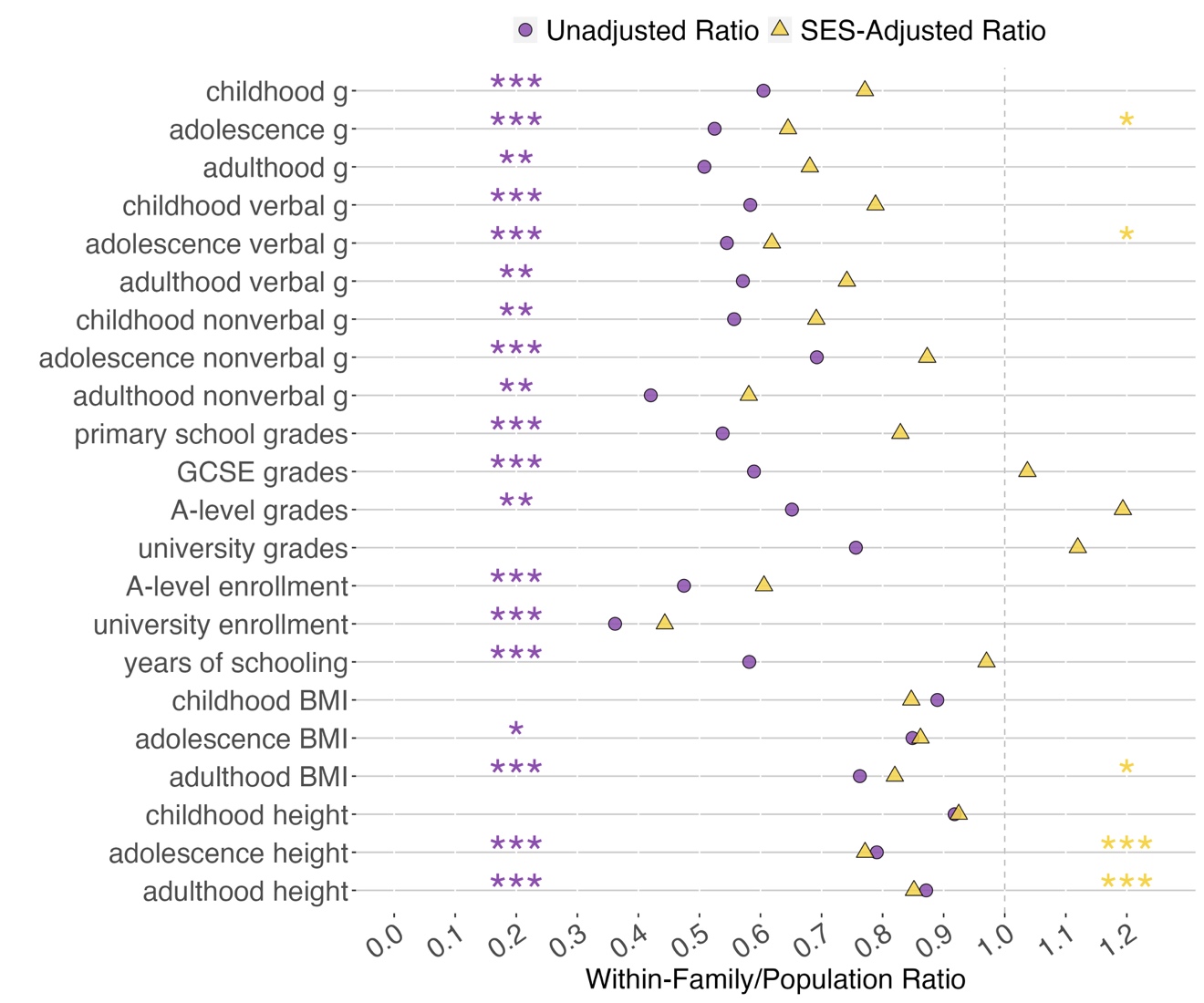
BF effects are greatly attenuated when SES is controlled
Phenotypic SES is substantially correlated with cognitive and educational traits, 0.27 on average (Figure F3 and Table G7). When we adjusted our regression model for SES among cognitive and educational traits, the average population estimate of 0.24 in Figure 2 was reduced to 0.17 in Figure F4. Across cognitive and educational traits and ages, the average WF estimate remained unchanged (0.13) because SES is a BF factor. As a result, the average ratio of the WF estimates to the population estimate increased from 57% before adjustment for SES (purple circles in Figure 3) to 78% after adjustment (yellow triangles in Figure 3). More specifically, for educational achievement and years of schooling, WF effects completely accounted for population estimates; in fact, some of the WF estimates slightly but not significantly exceeded the population estimates. These SES-adjusted results are detailed in Tables G8 and G9.
_and_adjuste.jpeg)
WF contributions are similar at the extremes of the distribution
Subsequently, we tested for nonlinearity by including a quadratic term for the polygenic score in the model to assess whether within-family and population effects were consistent across the PGS distribution. For cognitive and educational traits, we found no evidence of nonlinearity, indicating that both within-family and population genetic effects remained stable across the range of PGS values (Table G10). In fact, the variance explained by the linear model was generally comparable to, or higher than, that of the quadratic model. An exception was BMI among the anthropometric traits, where stepwise regression indicated a significantly better model fit (based on AIC) for the quadratic model; however, the increase in explained variance was minimal. Decile plots illustrating the relationship between PGS deciles and trait outcomes across traits and developmental stages are presented in Figures F5 to F11.
WF results are similar for females and males
In addition, we conducted sensitivity analyses to evaluate the robustness of our findings. For the population estimates, we compared outcomes between females and males and between MZ and DZ twins; for the WF estimates, we compared outcomes between same-sex females, same-sex males, and opposite-sex DZ twins. These comparisons showed no significant differences in the subset analyses for either the population or WF models, as illustrated in Figures F12 and F13.
Discussion
In this first systematic investigation of within-family (WF) PGS effects across cognitive and educational traits from ages 7 to 25, we found that WF PGS effects accounted for only about half of the population PGS effects for cognitive abilities from childhood to adulthood, for educational achievement from elementary school through high school, and for educational attainment in adulthood. This finding emerged even though PGS prediction increased by 50% from childhood to adolescence for cognitive abilities and educational achievement. As noted earlier, increasing heritability from childhood to adolescence and adulthood has been shown in twin studies (Haworth et al., 2010) and there is some evidence that PGS prediction also increases from childhood to adolescence (Selzam et al., 2017). This developmental increase in heritability for cognitive traits is generally interpreted in terms of genotype-environment correlation in the sense that genetic effects are amplified as individuals select, modify, and create environments correlated with their genetic propensities. Our finding suggests that this is the case for both WF and BF contributions to the PGS prediction in the population.
BF effects for cognitive and educational traits
Defining between-family (BF) effects as the gap between the WF and population PGS estimates, these findings for cognitive and educational traits point to an important role for BF factors whose effects are shared by siblings growing up in the same family and thus are not reflected within families. In contrast, for height and BMI, WF effects account for much more (84%) of their PGS prediction, suggesting that BF factors have much less effect on these traits.
We propose that the PGS prediction is stronger for cognitive and educational traits than for other behavioral domains such as psychopathology (Plomin, 2022) because cognitive and educational traits include BF effects in addition to WF effects, whereas psychopathology only includes WF effects. In support of this hypothesis, BF factors such as population stratification, assortative mating, and passive genotype-environment correlation affect cognitive and educational traits much more than psychopathology. For example, in our study, the quintessential stratification factor SES correlates 0.27 on average with cognitive and educational traits; SES correlates only 0.05 with psychopathology symptoms (Lin et al., 2024). After controlling for SES, WF PGS effects completely account for population PGS effects for educational achievement and attainment (Figure 3). However, we suggest that this finding is less informative than it seems at first glance. Because the major component of SES is educational attainment, it is almost tautological that the PGS for educational attainment accounts for less variance in educational achievement and attainment when familial SES is controlled, which only affects the BF component of PGS prediction. Indeed, our SES composite, measured at four developmental stages (birth, age 7, 16, and 21), correlated with the educational attainment polygenic score at an average of 0.37 (Table G11 and Figure F14), suggesting overlaps between SES and educational genetic predictors.
Population stratification factors other than SES, such as ancestral or geographical variation, might also contribute to the BF effects on cognitive and educational traits, as well as other BF factors such as assortative mating and passive genotype-environment correlation. For example, assortative mating is much greater for cognitive ability (spouse correlations ~ 0.40) and educational attainment (~0.50) than for psychopathology (~0.15) (Horwitz et al., 2023). Passive genotype-environment correlation, a double-barreled effect in which offspring passively receive parental environments correlated with the offspring genetic propensities, is also a BF factor because siblings share the same parents. Passive genotype-environment correlation has been reported to be substantial for cognitive abilities in childhood (Loehlin & DeFries, 1987).
BF effects and twin heritability estimates
One implication of finding substantial BF genetic effects for cognitive and educational traits is that the ‘missing heritability gap’ between PGS or SNP heritability and twin heritability is larger than assumed for cognitive and educational traits. Twin heritability estimates are about 50% for general cognitive ability, 55% for specific cognitive abilities, 60% for educational achievement, and 40% for educational attainment (Procopio et al., 2022). From the earliest DNA studies of cognitive and educational traits, SNP heritability accounted for half of the twin heritability estimates (Plomin et al., 2013). PGS and SNP heritabilities include BF genetic effects because they are derived from unrelated individuals reared in different families. However, in twin studies, BF genetic effects result in underestimates of heritability for cognitive and educational traits because the twin design only detects WF genetic variance. Twin analyses misread BF genetic variance as environmental influence shared by twins, labeled C (‘common’) in the ACE twin model in which A refers to additive genetic variance and E is nonshared environmental variance (Knopik et al., 2017). Because twin studies underestimate heritability when BF genetic effects are present, the gap between PGS or SNP heritability and actual heritability is likely to be larger than previously assumed for cognitive and educational traits (Plomin & von Stumm, 2018). In other words, the ceiling for PGS and SNP heritability might exceed twin heritability.
BF effects are not ‘bias’
Genetic variance in the population generally segregates within families, but for cognitive and educational traits, between-family genetic variance also contributes to the population variance. Distinguishing WF and BF effects can be useful. For example, predicting sibling differences in a trait depends on WF effects, and finding BF effects leads to research on factors such as population stratification, assortative mating, and passive genotype-environment correlation (Howe et al., 2022; Okbay et al., 2022). However, an unfortunate trend is to refer to WF effects as ‘direct’ and BF effects as ‘indirect’ or, worse, as confounded, spurious, inflated, and biased. Indeed, it could be argued that WF effects are biased because they miss BF effects that can predict differences among unrelated individuals in the population. Moreover, WF effects are no more direct than BF effects. Both WF and BF PGS associations with traits can be mediated by correlations between genotypes and environments. Although WF effects do not include passive genotype-environment correlation, WF as well as BF effects are mediated by the more general processes of reactive (evocative) and active genotype-environment correlation (Plomin et al., 1977).
We suggest that such pejorative interpretations of bias are misguided from the perspective of prediction rather than explanation and that the major application of PGS will be to predict genetic propensities of unrelated individuals in the population (Plomin & von Stumm, 2022). We argue that BF effects are legitimate sources of genetic variance for the prediction of individual differences in a particular population for practical as well as conceptual reasons. It is not feasible to separate children from their parents to avoid passive genotype-environment correlation, or to make couples mate randomly to avoid assortative mating. We cannot realistically remove SES differences to eliminate population stratification. Moreover, all genetic variance is ultimately ancestral.
Passive genotype-environment correlation, which occurs when children passively inherit from their parents’ family environments that are correlated with their genetic propensities, is a between-family effect because children in a family have the same parents. However, two other types of genotype-environment correlation are more general and can operate both within and between families. Evocative genotype-environment correlation occurs when individuals evoke reactions from other people, not just relatives, on the basis of their genetic propensities. Even more general is active genotype-environment correlation which appears when individuals select, modify, or create experiences that are correlated with their genetic tendencies. These general processes of the interplay between genotype and environment extend beyond the individual to shape both within-family and between-family variations. It aligns with Dawkins’ extended phenotype concept, where genetic effects manifest through environmental modifications (Dawkins, 1982). In the case of genotype-environment correlation, the focus is on how individuals’ genetically influenced behaviors and traits shape their own developmental contexts, creating feedback loops that amplify phenotypic variance. Critically, between-family effects like passive genotype-environment correlation are not statistical noise but reflect real, population-level processes that contribute to prediction.
The use of terms such as bias denigrates the predictive power of PGS and detracts from the motivation needed to launch bigger and better genome-wide association studies of unrelated individuals to enhance PGS predictive power in the population. We suggest that WF and BF effects be labeled operationally as within-family and between-family, rather than using pejorative labels like ‘bias’ that favor one component of population variance over the other.