Genes, Environments, and the Development of Intelligence in Children of Mothers With Phenylketonuria

1. Introduction

Children of mothers with phenylketonuria (PKU) offer an intriguing look at the interplay of genetic and environmental factors that influence the development of intelligence. Most simply, PKU has a genetic basis. PKU results from mutations on the phenylalanine hydroxylase (PAH) gene, mutations that impede the metabolism of phenylalanine (PHE) into tyrosine. PKU is a recessive trait, so an individual must be homozygous for mutations on the PAH gene to have PKU. Homozygosity means that a person receives mutations on the PAH gene from both parents. In contrast, heterozygosity, which refers to receiving a PAH gene mutation from one parent but a non-problematic PAH gene from the other parent, results in an individual being a carrier of the genetic basis of PKU, but not subject to the teratogenic effects associated with PKU, as they will be able to metabolize PHE normally. Over 1,500 different mutations on the PAH gene have been identified, many of which have been assessed for severity of the mutation (see https://databases.lovd.nl/shared/genes/PAH).

Children with PKU appear normal at birth, so their status as having PKU is typically identified with the Guthrie test (Guthrie, 1961; Kuehn, 2013), a blood test employing a heel stick within the first week or two after birth. If a child with PKU is on a normal diet, the buildup of PHE in their blood leads to brain damage and a mean IQ of about 50 by age 2 years, a decline in IQ that is not remediable. Conversely, if the child with PKU is put on a PHE-restricted diet within the first two weeks or so after birth and remains on the diet through the developmental period, normal intellectual development can be expected. Thus, PKU is a “poster child” syndrome for the fact that high heritability need not imply destiny. That is, prior to development of the Guthrie test, heritability of the low-IQ PKU phenotype was extremely high; persons with PKU were often identified too late to avert the teratogenic effects of high PHE levels in their blood, leading to very low levels of IQ. But, with the early diagnosis afforded by the Guthrie newborn screening test, children with PKU could receive a crucial environmental manipulation – being put on a low-PHE diet – very early in life. If this were done, the negative effects of their genetic mutations could be countered, normal intellectual development could ensue, and the heritability of the PKU-related low-IQ phenotype fell to very low levels in the 1960s.

Children of mothers with PKU receive a genetic mutation on the PAH gene from their mother. But, due to the lack of assortative mating for PAH mutation, the vast majority of children of mothers with PKU receive a non-problematic PAH gene from their fathers, so do not have PKU. However, during gestation, if the pregnant mother is on an unrestricted diet, the buildup of PHE in her blood passes the placental barrier and can harm the developing fetus. In an early review of offspring outcomes from 524 untreated pregnancies by 155 women with PKU, Lenke and Levy (1980) documented negative outcomes in a wide array of offspring characteristics if the women were not on a low-PHE diet during pregnancy. For example, exposure of the fetus to high prenatal levels of PHE led to increased risks of mental retardation (now termed intellectual disability, or ID), microcephaly, congenital heart disease, and low birth weight, and the effects of exposure to PHE appeared to follow a dose-response function for each outcome variable. Thus, 92% of offspring of mothers with high levels of PHE (≥ 20 mg/dL, or ≥ 1200 μmol/L)^[1] met an IQ < 75 cutoff for ID, whereas only 21% of offspring of mothers with moderate levels of PHE (3 ‒10 mg/dL, or 180 ‒ 600 μmol/L) met the same criterion. But this rate of 21% meeting the low IQ cutoff for offspring of the least affected mothers with PKU still exceeds considerably the 5% of offspring with IQs < 75 that would occur in a representative sample from the population. Hence, even the relatively low levels of exposure to PHE for offspring of mothers in the lowest exposure group (3 ‒ 10 mg/dL) led to notable increases in rates of low intelligence over the rate expected in the population.

Despite considerable research reporting detrimental effects of prenatal phenylalanine exposure, much remains to be determined concerning effects of prenatal exposure to PHE on offspring developmental outcomes. One theoretical concern is the form of the relation between prenatal PHE exposure and offspring outcomes and the associated safe level of PHE exposure. Safe levels of average PHE exposure have been disputed for decades, with some experts arguing for levels of 6 mg/dL or less (360 μmol/L or less) (e.g., Adams et al., 2023; Grohmann-Held et al., 2022; Nielsen et al., 2023), whereas others found few problems with much higher levels (e.g., 18 mg/dl in Lenke & Waisbren, 1983). Recently, Widaman and Helm (2024) fit linear and two-piece linear spline models to data on maternal PHE levels during pregnancy and several infant and child intelligence outcome measures. They found that two-piece linear spline models were more strongly related to outcomes than were standard linear models. Across a range of intellectual, language, and adaptive functioning outcomes, the mean threshold for teratogenic effects of PHE exposure was between 6 and 7 mg/dL. So, if an infant was exposed to less than 6 or 7 mg/dL, on average, during gestation, no detrimental effects of PHE exposure were evident. But, if the child was exposed to average PHE concentrations greater than 6 or 7 mg/dL, the spline model documented an approximate 4-point IQ drop for every 1 mg/dL increase in average PHE exposure above the threshold point.

Parental background factors. Given superior fit of two-piece linear spline models to represent relations between PHE exposure and child outcomes, a further key question – and the one motivating the current research – involves the relative impact of prenatal exposure to PHE on child outcomes when estimated in the context of other relevant predictor variables. One obvious predictor of offspring intelligence is parental intelligence (Sattler, 2001). Effects of parental intelligence are easy to justify, as parents contribute to their offspring both genetic material and various forms of environmental stimulation that presumably affect offspring intelligence. Behavior genetic studies often conclude that over half of the variance of intelligence scores is associated with genetic factors, with environmental factors explaining much smaller amounts of variance (e.g., McGue & Bouchard, 1998).

Parental socioeconomic status (Bradley & Corwyn, 2002) and parental education (Broman et al., 1987) are also strong correlates or predictors of offspring intelligence throughout infancy, childhood, and adolescence and thus appear to be reasonable influences on offspring outcomes. Advocates of genetic explanations of intelligence often argue that effects of socioeconomic status and education of the parents on childhood outcomes are largely indirect effects of genetic sources of variance: parents with more favorable genetic endowments not only have higher intelligence, but also tend to have higher socioeconomic and education levels and provide more stimulating home environments.

One potentially important background variable – unique to the study of offspring of mothers with PKU – is the severity of the mother’s PAH mutation. As explained by Güttler et al. (2003), mothers with PKU are classified with regard to the severity of their PAH mutation, based on a PHE loading test. In such a test, an individual ingests food with a certain amount of PHE, and blood is drawn after a standard time interval to determine the level of PHE in the blood. The higher the amount of PHE in the blood, the more severe the mutation, as less PHE has been metabolized into tyrosine. The level of PHE in blood after a test, termed the individual’s assigned PHE level, often leads to groupings of: (a) classical PKU, with PHE > 20 mg/dL (> 1200 μmol/L); (b) moderate PKU, with PHE 15 – 20 mg/dL (900 – 1200 μmol/L); (c) mild PKU, with PHE 10 – 15 mg/dL (600 – 900 μmol/L); and (d) mild hyperphenylalaninemia (MHP), with PHE 3 – 10 mg/dL (180 – 600 μmol/L). After specific genetic mutations were identified, Güttler and Guldberg (2000) developed a numerical system, with higher numbers indicating less severe mutation. Mothers with more severe PAH mutations would likely have greater difficulty maintaining low blood PHE levels during pregnancy, which would create a more teratogenic intrauterine environment for the developing fetus. But, when predicting offspring birth and childhood outcomes, the importance of the severity of the mother’s PAH mutation has never been established, especially within the context of other important background variables such as mother’s IQ, SES, and education.

Pregnancy variables. In addition to genetic and postnatal environmental sources of variance in the general population, prenatal exposure to PHE is yet another factor that may influence offspring cognitive outcomes (Denniston, 1963; Kirkman & Hicks, 1984; Lenke & Levy, 1980; Smith, Beasley, et al., 1990). Most research on maternal phenylketonuria has attempted to document the relation between maternal blood PHE levels during pregnancy and child outcomes, but has failed to estimate these effects within larger or more inclusive models for child developmental outcomes. That is, mothers with higher blood levels of PHE during pregnancy may also have lower levels of intelligence, SES, and education. Hence, maternal intelligence, SES, and/or education may be as important or even more important than PHE levels during pregnancy when predicting offspring cognitive outcomes.

Other pregnancy-related variables could also influence infant cognitive outcomes. For example, protein is a building block of many organ systems, including the brain. Thus, maternal intake of protein during pregnancy may enhance the growth and development of the fetus in multiple ways (Linderkamp & Linderkamp-Skoruppa, 2021; Rushmore et al., 2022; Tonkiss et al., 1993; Zamenhof & van Marthens, 1974). Weight gain during pregnancy and duration of the gestation may also influence infant and child outcomes. Low levels of weight gain during pregnancy can lead to small-for-gestational-age status, which is negatively related with cognitive test performance from infancy into adulthood (e.g., Christian, Murray-Kolb, Tielach, Katz, LeClerq, & Khatry, 2014; Eves et al., 2020). Whether length of gestation/preterm birth has significant effects on intelligence is less clear (e.g., Christian et al., 2014), but length of gestation should be assessed for possible effects on infant and child functioning.

Infant birth status. Infant perinatal status could mediate effects of maternal background and pregnancy-related variables on infant IQ. The three indices of infant perinatal status available in the current study were birth weight, length, and head circumference. Birth weight and length are highly correlated indices of neonatal status, with heavier weight and longer length, within limits, indicating physically more robust neonates, and these measures are related to intelligence in childhood (Kirkegaard et al., 2020) and later (Flensborg-Madsen et al., 2020). Further, low birthweight has long been associated with negative intellectual performance (see reviews by Gu et al., 2017; Shenkin et al., 2004).

Birth head circumference is another key predictor of cognitive outcomes, with birth head circumference positively related to intelligence in childhood (Bach et al., 2020; Kirkegaard et al., 2020). Research by Qian, Gao, Yan, Yang, Wang, Bai, Ma, and Yang (2021) indicated that birth head circumference was a much stronger correlate of later intelligence than were birth weight and length. Small birth head circumference, often indexed as the presence of microcephaly, is a frequent predictor of poor later cognitive performance (Leibovitz et al., 2022).

The present study. The primary goal of the present study was to examine the relative effects of prenatal PHE exposure on offspring cognitive outcomes within the context of a rich set of alternative potential predictors of those outcomes. This set of potential predictors included several maternal background variables (maternal SES, education, IQ, age, and severity of PKU mutation), pregnancy-related variables (weight gain, PHE level, PHE variability, weeks gestation, and protein intake), and indicators of perinatal status (birth length, weight, and head circumference). The current study is an extension of prior work by Widaman and Azen (2003), using more complete data and additional indicators that were not available for that earlier study.

A schematic rendition of our modeling project is shown in Figure 1, which contains four sets of variables. Set X contains five background variables that are hypothesized to have effects on the four child intelligence outcomes shown as Set Y. In addition to these two sets of variables, two sets of potential mediators are shown in Figure 1. The first of these, identified as Set M1 includes five pregnancy-related variables, and the second, listed as Set M2 contains two birth outcome variables. After demonstrating that Set X variables have significant effects on Set Y child outcomes, it will be important to determine whether Set X variables have effects on the mediators in Sets M1 and M2. Then, we will investigate whether the mediators in Sets M1 and M2 have significant relations with child outcomes in Set Y and thereby mediate fully or partially the effects of Set X variables on the outcomes in Set Y.

Figure 1.Conceptual mediation model showing background characteristics (Set X), prenatal mediators (Set M1), birth outcome mediators (Set M2), and child intellectual outcomes (Set Y).

2. Method

2.1. Participants

The Maternal PKU Collaborative Study began in 1984 as a prospective study to evaluate the effects of diet during pregnancy on offspring characteristics. Children’s Hospital of Los Angeles was the Coordinating Center and was one of the four regional Contributing Centers in the United States, along with one center in Canada and one in Germany, that recruited participants at a total of 78 Participating Centers. Enrollment of participants occurred from 1984 through 1996 (see Koch et al., 2003, for further details).

All women with PKU who were known to metabolic clinics in the United States, Canada, and Germany were enrolled in the study when they became pregnant. For women with PKU, dietary treatments were employed to keep their blood PHE levels during pregnancy between 2 and 6 mg/dL. Women with mild hyperphenylalaninemia (MHP), defined as blood PHE levels less than 10 mg/dL on a normal diet, were also invited to participate in the study, although dietary treatments were not used with these women. Virtually all pregnant women with PKU or MHP agreed to participate in the study.

The final study sample consisted of 572 pregnancies, of which 413 resulted in live births. Among the remainder were 75 spontaneous abortions, 78 elective abortions, 3 stillbirths, and 3 others (2 children with PKU, 1 child with parental refusal to participate). All pregnancies were monitored systematically, with blood PHE levels and dietary intake assessed weekly, visits to a metabolic center (enabling assessment of nutrition status, weight gain, and amino acid levels) once each trimester, three ultrasound examinations, and regular obstetrical visits. Offspring were assessed at birth and then at ages 1, 2, 4, and 7 years of age.

2.2. Latent Variables and Their Manifest Indicators

Manifest variables for current analyses are listed in Table 1, with the descriptive statistics of number of participants with available scores, mean, SD, and minimum and maximum values.

2.2.1. Set X: Background Variables

Five demographic, or background, latent variables on the mothers included in the study were specified in structural models. The first background latent variable was Socioeconomic Status (SES) of the household in which the mother resided, which was a single-indicator latent variable. This indicator was derived from the Hollingshead two-factor index of SES for the head of the household. Hollingshead scores were left in continuous form, ranging from 11 to 77, with higher scores indicating lower socioeconomic status. As shown in Table 1, the mean score was 51.30 (SD = 14.73), so the average mother resided in a lower middle-class home. Hollingshead scores were then reversed, so higher scores reflected higher levels of SES, for ease of interpretation in our statistical analyses.

The second background latent variable, Maternal Education, had a single indicator, scored on a Likert-scaled continuum, with scale points (after reverse scoring) ranging from 1 = “less than eighth grade” to 7 = “post graduate or professional degree,” so that higher scores indicated more years of education. Participants had a mean score of 4.09 (SD = 1.09), where 4 = “high school graduate.”

The third background latent variable was Maternal Intelligence, which had two indicators: the Verbal IQ and Performance IQ scores from the Wechsler Adult Intelligence Scale – Revised (Wechsler, 1981). As shown in Table 1, the sample of mothers had mean Verbal and Performance IQs of 85.6 and 88.5, respectively; for reference, Table 1 also shows that the mothers had a mean Full Scale IQ of 85.9. Thus, the sample of mothers fell, on average, about one SD below the population mean on intelligence. The relatively low mean SES of mothers, reported above, is consistent with the relatively low mean IQ of mothers in this sample.

Maternal Age at conception (in years) was the fourth demographic latent variable. As shown in Table 1, maternal age at conception ranged from 16 to 36 years, with a mean of 24.1 years (SD = 4.06), so mothers in the sample tended to have offspring at a relatively early age.

The fifth background latent variable, Severity of Mutation, reflected the severity of the genetic mutation on the mother’s PAH gene. Severity of Mutation was assessed by two variables: (a) maternal assigned or tested PHE level, which is an index of blood PHE level (in mg/dL) after a PHE loading test, and (b) a score developed by Güttler and Guldberg (2000) that represents the severity of the mutation on the PAH gene. For the assigned PHE level indicator, higher scores indicate higher levels of blood PHE after a PHE loading test, which in turn represents a more severe mutation, as less phenylalanine is converted into tyrosine. As shown in Table 1, the mean assigned PHE level of 22.03 mg/dL (SD = 9.18) fell in the classical PKU range (i.e., > 20 mg/dL), and there was wide variability in these scores. The Güttler score can range from 2 to 16, with higher numbers reflecting milder mutations. The sample of mothers had a mean Güttler score of 4.0, indicating relatively severe mutational status.

2.2.2. Set M1: Pregnancy-related variables

Five pregnancy-related latent variables were specified in the structural models for this paper. The first was Weight Gain during pregnancy, which had two indicators: (a) weight gain (in lbs) during pregnancy, and (b) percent of recommended weight gain. For both, higher scores indicated greater weight gain during pregnancy. The sample of mothers gained an average of 29.0 lbs during pregnancy, but showed wide variability in weight gain (from –13 to 70 lbs). Expressed as percent of recommended weight gain, mothers gained an average of about 36% more weight than recommended, with a wide range of scores (from –86 to +455 %).

The second pregnancy-related variable was protein intake per day during pregnancy (in gm). On average, mothers in the study ingested a moderate amount of protein (M = 74.5 gm), but considerable individual differences in protein intake occurred (SD = 18.6 gm).

The third pregnancy-related variable was PHE Level, which was assessed using two indicators: (a) average PHE level, which was the simple average of all levels recorded during the pregnancy; and (b) the week during pregnancy when all remaining PHE levels were less than 10 mg/dL. On both indicators, lower scores indicated better control of dietary PHE. On average, mothers maintained fairly good control of PHE level (M = 8.23 mg/dL), although the range of average PHE levels (from 1.3 to 28.3 mg/dL) showed that some mothers had very good, low levels, whereas others had average PHE levels far beyond recommended levels. Note that we also report average PHE levels in μmol/L units, for reference. Widaman and Helm (2024) found that teratogenic effects of PHE exposure begin at PHE levels around 6 mg/dL, so we created a new variable, identified in Table 1 as ‘Pregnancy PHE level > 6 mg/dL,’ which is simply the number of mg/dL of average PHE over 6 mg/dL. Thus, on this variable, all individuals with average PHE levels below 6 mg/dL would have scores of zero. On the variable indexing timing of control below a given PHE level, the values shown in Table 1 reveal that some mothers were in good PHE control prior to conception (i.e., those with values of 0), whereas others never gained good control of PHE levels during pregnancy.

The fourth pregnancy-related variable was PHE variability during pregnancy, assessed by the standard deviation of PHE levels (SD PHE) for all tests during pregnancy (cf. Maillot et al., 2008). The protocol for mothers in the MPKU study called for monitoring PHE levels at least every two weeks of pregnancy. On average, mothers in the study had their PHE levels assessed about 16 times during pregnancy and showed moderate fluctuations in their PHE levels (M = 2.75 mg/dL, SD = 1.50).

The fifth pregnancy-related variable was Weeks Gestation of the pregnancy, ranging from about 28 to 43 weeks (see Table 1). On average, mothers had pregnancies of typical length (M = 39.2 weeks), with modest variability in length of pregnancy (SD = 1.9 weeks).

2.2.3. Set M2: Birth outcome variables

Two birth-related latent variables were specified in the structural models. The first latent variable was Birth Size, with two indicators: birth length (in cm), and birth weight (in gm). Values shown in Table 1 reveal moderate average birth length (M = 49.0 cm) and birth weight (3069 gm), but fairly wide variability in both indicators. For analyses, birth weight was divided by 1000, to provide birth weight in kg, to make the mean and SD of birth weight more similar in magnitude to other variables. Statistics for birth weight in kg are also shown in Table 1.

The second latent variable, Birth Head Circumference, had a single indicator: birth head circumference (in cm). The mean head circumference was 32.8 cm, with moderate variability (SD = 1.95 cm) around this value. World Health Organization standards for birth head circumference^[2] yield M = 34.2 cm and a value of 33.0 cm as 1 SD below the population mean. Thus, the mean head circumference in our sample was just over 1 SD below the population mean. But, relatively small head circumference is consistent with prior studies of children of mothers with PKU, which often report mean head circumference around 33.0 cm (Drogari et al., 1987; Fiellet et al., 2004; Lee et al., 2003, 2005; Naughten & Saul, 1990; Smith, Glossop, et al., 1990).

In addition to standard measures of birth status, each of the three birth measures were converted to z-scores using population norm tables. These transformations yielded scores that were more easily interpreted in relation to population norms and also contained a correction for gestational status. As shown in Table 1, neonates in the study had mean birth lengths that were about one-third SD below the population norm (M = –0.32) and mean birth weights that were over one-half SD below the population norm (M = –0.62). The neonates were even farther below the population norm on birth head circumference, exhibiting a mean that was over 1 SD below the population (M = –1.02). Because these z-score measures were corrected for gestational status, the sample of infants in this study showed considerable growth retardation at birth, presumably due to the detrimental intrauterine environments to which they were exposed.

2.2.4. Set Y: Offspring cognitive outcomes

The measures of infant intelligence or cognitive status used in the present study were obtained at offspring ages 1, 2, 4, and 7 years of age. At 1 and 2 years of age, three manifest variables were obtained at each time of measurement: the Mental Development Index (MDI) from the Bayley Scales of Infant Development (Bayley, 1993), and the Receptive Language Quotient and Expressive Language Quotient from the Receptive-Expressive Emergent Language (REEL) test (Bzoch & League, 1970, 1991).

At the 4 year assessment, the three manifest indicators used in analyses consisted of: the General Cognitive Index (GCI) from the McCarthy Scales of Children’s Abilities (McCarthy, 1972), the Composite Spoken Language Quotient (CSLQ) from the Test of Language Development (TOLD; Newcomer & Hammill, 1991), and the Communication domain score from the Vineland Adaptive Behavior Scales (VABS; Sparrow et al., 1984). Then, at the 7-year assessment, the Verbal IQ and Performance IQ scores from the Wechsler Intelligence Scale for Children – Revised (WISC-R; Wechsler, 1974) were the two manifest indicators of intelligence status.

Standardized scores were obtained for each of the 11 manifest indicators using norm tables from the various tests. All tests had been normed to yield a mean of 100 and SD of 15 in the population. All scores had strong psychometric properties, with all reliabilities above .85 and most above .92.^[3]

2.3. Analytic Procedures

Estimation. When fitting structural equation models to data, we used the Mplus program (Muthén & Muthén, 1998–2017). Due to the presence of missing data, we used full information maximum likelihood (FIML) estimation of model parameters. FIML estimation involves fitting structural models directly to raw data, with missing values identified using a missing data indicator. FIML estimation has been found to be an efficient and unbiased method of estimation in the presence of missing data when data are “missing at random” and is perhaps the best alternative to use even if data do not meet the “missing at random” assumption. In the present study, missing data occurred for several reasons, such as a family moving far from a participating center. Given reasons for missing data, characterizing the missing data as “missing at random” seems appropriate, and FIML estimation is highly appropriate for such applications.

Model identification. For all structural models, we identified the scale for each latent variable with multiple indicators by fixing the latent variable variance to unity, fixed all latent variable means to zero, and estimated all manifest variable intercepts. For single-indicator latent variables, we fixed the factor loading to unity and fixed the unique factor variance to zero. For latent variables with two or more indicators, we estimated all factor loadings and unique variances. After arriving at a final, acceptable model, we reported rescaled parameter estimates from a standardized model in which all latent variables were transformed to have unit variance. As is common practice, any parameter estimate that, when divided by its standard error (SE), had a critical ratio of 2.0 or greater was considered statistically significant.

Assessment of model fit. Model fit was evaluated using both the likelihood ratio χ² goodness of fit statistical test and practical fit indices. The traditional χ² index is a test of exact fit of a model to data. With a large sample size, the χ² test of exact fit is often overly sensitive, and thus prone to yield a significant test statistic value, even in the presence of minor levels of model misfit. Due to the relatively large sample size and the large number of tests computed, we used the .01 level when evaluating indices of difference in model fit.

Given oversensitivity of the χ² test, three other fit indices were used. The first practical fit index was the Root Mean Squared Error of Approximation (RMSEA). Values of the RMSEA below .05 indicate close fit to the data, values between .05 and .08 moderate fit, values between .08 and .10 poor fit, and values over .10 unacceptable fit. Accompanying use of the RMSEA is a 90% CI; if the lower limit of the CI is less than .05, close model fit cannot be rejected. The second practical fit index was the Tucker-Lewis Index (TLI; Tucker & Lewis, 1973), which is an index of the proportion of explainable off-diagonal covariation explained by a model. TLI values over .95 indicate close fit of a model. The third fit index was the standardized root mean squared residual (SRMR) correlation, with values below .08 preferred.

When comparing nested models, we report the χ² difference test, which is the difference in χ² values for the two models (Δχ²), which is distributed approximately as χ² with degrees of freedom equal to the difference in degrees of freedom (Δdf) for the two models. We report the change in the TLI and SRMR measures; negative values of the ΔTLI and positive values of the ΔSRMR indicate worse fit for the more restricted model. Based on recent work by Savalei, Brace, and Fouladi (2024), we also report the RMSEA_D, which is an RMSEA based on the Δχ² and the Δdf for the two models. First proposed by Browne and Du Toit (1992), RMSEA_D values fall on the same scale as RMSEA values, so values lower than .05 indicate close fit of the restricted model relative to the more highly parameterized model, etc. See Supplemental Material at https://osf.io/kwtc6/ for more information, including a program to estimate RMSEA_D and its CI based on Raykov and Penev (1998).

Analytic strategy. We used a conservative, “less is more” model fitting strategy, keeping the number of significance tests to a minimum, given the size of the model. We operationalized this strategy as follows: When testing effects of one set of variables (e.g., Set X) on another set of variables (e.g., Set Y), we compared the fit of two models – one model that estimated all possible directed paths from latent variables in the first set to latent variables in the second set, and a second, nested model in which all direct paths between latent variables in the two sets were fixed at zero. This allowed a setwise test of the statistical significance of the entire set of path coefficients using a single χ² test. If the model comparison showed no or trivial worsening of fit when fixing all path coefficients to zero, the second, more restricted model was deemed the better model, given its greater parsimony and approximately equal levels of fit. If the model comparison revealed an unacceptable worsening of model fit, we then altered the more restricted model by freeing up directed path coefficients based on a priori theory and significance of path coefficients in the less restricted model. This modified model was then compared with both of the preceding models to determine its relative fit to the data.

Regarding magnitude of effects, we followed Funder and Ozer (2019) in interpreting correlations of .10, .20, .30, and .40 as small, medium, large, and very large effects, respectively. Recent work by Orth, Clark, Donnellan, and Robins (2021) suggests that prospective (i.e., across time) standardized lagged regression weights in longitudinal models between .10 and .20 in absolute magnitude are relatively large, so values above .20 are quite large.

For two primary reasons, we did not pursue a latent growth curve analysis of the intelligence measures, which would have taken the form of summarizing intelligence measures across ages 1 to 7 years using a latent intercept and slope(s), and then predicting the latent intercept and slope(s) using sets X, M1, and M2. First, because all intelligence measures were normed separately at each age, mean changes over time were not expected, making a slope latent variable suspect. Second, the content of intellectual assessments at 1 or 2 years of age, which is primarily perceptual/manual and non-verbal, is extremely different than content in intelligence assessments in childhood, which is largely verbal, similar to measures in adolescence and adulthood. Growth curve methods require the assumption that the same measure is obtained across times of measurement, which could not be supported in the current analytic context. Despite evolving age differences in test content, standing on an intelligence measure at one age is the best predictor of standing on an intelligence measure at the next time of measurement. Therefore, an autoregressive model was pursued for the longitudinal measures of intelligence.

3. Results

3.1. Correlations among Manifest Variables

Correlations among the 28 manifest variables included in the mediation model are shown in Table 2.^[4] The first seven variables were indicators of the background latent variables and had expected patterns of correlation. Maternal SES, education, and intelligence measures were all substantially positively correlated, and maternal age at conception was modestly positively correlated with these variables. The sixth variable, labeled ‘M tested PHE’ which was the mother’s PHE level after a PHE loading test, was negatively correlated with other background variables, as higher scores on this variable indicated more severe PAH gene mutation, so mothers with more severe mutations tended to have lower SES, education, and intelligence scores.

Variables 8 through 10, from SD PHE through Week < 10 mg/dL, were pregnancy variables for which higher scores were associated with poorer blood PHE control. As a result, these variables tended to correlate negatively, as hypothesized, with most other variables. Variables 11 through 17 included remaining pregnancy variables and birth outcome variables, and these tended to have modest to moderate correlations with other variables in the matrix.

Of considerable interest are the correlations of background, pregnancy, and birth measures with cognitive outcomes (cognitive outcomes are variables 18 through 28). As expected, maternal background variables tended to have moderate to strong correlations with cognitive outcomes, ranging from about .10 to .45. The indicators of PHE level during pregnancy (variables 8, 9, and 10) had rather stronger correlations with cognitive outcomes, ranging from ‒.18 to ‒.69, with a median of ‒.49. The remaining pregnancy variables (variables 11 through 14) tended to have more modest correlations with cognitive variables. The birth outcome variables (variables 15 through 17) had moderate to strong correlations with the cognitive outcomes. Replicating prior research (e.g., Drogari et al., 1987; Qian et al., 2021), birth head circumference had stronger correlations with cognitive outcomes, ranging from .35 to .49, than did birth length or weight. The cognitive variables were all strongly mutually correlated.

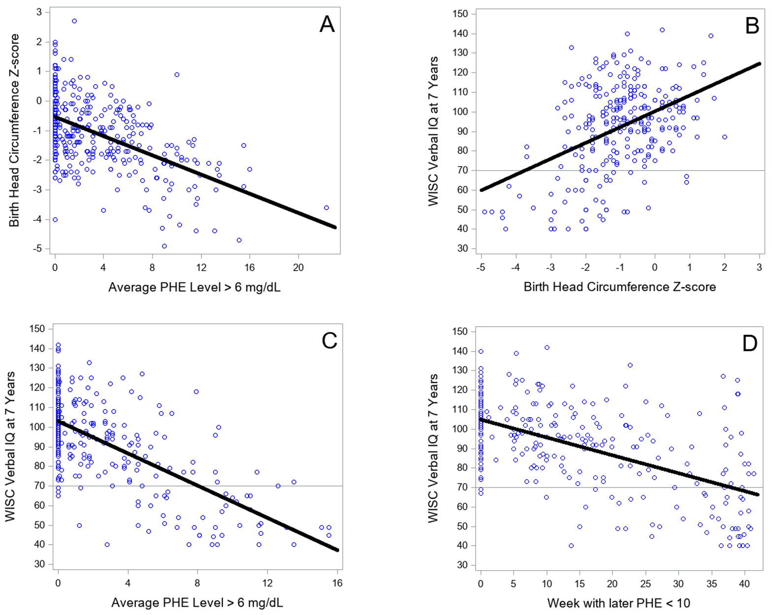
Many of the correlations in Table 2 appeared to be rather large, particularly correlations between biological variables and intelligence outcomes. At the request of a reviewer, four scattergrams in Figure 2 demonstrate that the high correlations were not positively biased in magnitude from undue influence by outliers. Figure 2A shows the relation between PHE level > 6 mg/dL and birth head circumference, r = ‒.53. A single outlier is notable, with a PHE level of 22.3 mg/dL, with the next lower PHE level being 15.5 mg/dL. Deleting this single outlier left the correlation between the two variables virtually unchanged, r = ‒.52. Figure 2B illustrates the relation between birth head circumference and WISC Verbal IQ at 7 years, r = .45. Figure 2C shows the relation of PHE level > 6 mg/dL with Verbal IQ at 7 years, r = ‒.66. Finally, Figure 2D shows the relation between week during pregnancy with all later PHE levels < 10 mg/dL and Verbal IQ at 7 years, r = ‒.56. None of the latter three panels of Figure 2 contained outliers that were likely to affect the magnitude of correlations among variables. Additional scattergrams of PHE > 6 mg/dL with each of the cognitive outcomes at all age levels are presented in Supplemental Material at https://osf.io/kwtc6/ ; none exhibited outliers.

Figure 2.Scattergrams, with fitted linear functions, for select pairs of variables. A. Birth head circumference as a function of average PHE > 6 mg/dL. B. WISC Verbal IQ at 7 years as a function of birth head circumference. C. WISC Verbal IQ at 7 years as a function of average PHE > 6 mg/dL. D. WISC Verbal IQ as a function of week during pregnancy with all later PHE levels below 10 mg/dL.

3.2. Testing Relations of X (Background Variables) with Y (Child Outcomes)

Prior to evaluating effects of proposed mediating variables, the first task was to verify the significance of relations between the initial or background latent variables (Set X) on the child outcome latent variables (Set Y). Thus, we fit competing models to data using variables from Sets X and Y shown in Figure 1. A total of nine latent variables were included in these models, five from Set X and four from Set Y. The five latent variables from Set X were SES of the home in which the mother resided, Maternal Education, Maternal IQ, Maternal Age at conception, and maternal Severity of PKU Mutation. As described above, Maternal IQ and Severity of Mutation each had two indicators, and the remaining latent variables had single indicators. The four latent variables from Set Y were Child Intelligence Status at 1, 2, 4, and 7 years; all four of these latent variables had multiple indicators.

Indices of fit of models tested in this section are shown in Table 3, and differences in model fit are shown in Table 4. The first model specified, Model 0, was a model with a saturated structural model, so allowed correlations among all nine latent variables. This model is a useful baseline model, and had acceptable fit, with a significant statistical index of fit, χ²(101) = 146.84, p = .002, but levels of practical fit that indicated close model fit to the data, with RMSEA = .033 and TLI = .978. These indicators of close fit of the model to the data suggest that the formations of the latent variables imposed by the model could not be rejected by the data (i.e., the latent variables provided a more parsimonious representation of the data as compared to a model with only manifest variables). Correlations among the latent variables are shown in Table 5. As expected, Maternal SES, Education, and IQ were all strongly positively correlated, Maternal Age was less highly correlated, and Maternal PKU Severity tended to be negatively associated with other background variables, especially Maternal IQ. The four child outcome variables were strongly intercorrelated and exhibited a simplex pattern, with highest correlations just off the diagonal and weaker ones further off the diagonal. Of note, 17 of the 20 correlations of background latent variables with child outcome latent variables were fairly large, ranging from .24 to .50 in absolute magnitude, and significant at p < .001, 2 correlations were significant at p < .05, and only a single correlation failed to reach statistical significance (p = .07). These correlations are important because they represent, individually, the total effect of each predictor latent variable on each outcome latent variable, and these correlations tended to be relatively large and statistically significant.

The first substantive model, termed Model 1, was a nine-factor model with correlations estimated among all five background latent variables, a total of 20 directed paths from each background latent variable to each outcome latent variable, and a first-order autoregressive pattern fit among the outcome latent variables. As shown in Table 3, Model 1 had very good levels of fit statistically and practically (e.g., RMSEA = .033 and TLI = .979) and fit non-significantly different than Model 0, with Δχ²(3) = 3.05, p = .38, and RMSEA_D = .006 (see Table 4). Parameter estimates from Model 1 are provided in the top half of Table 6, which shows that only 10 of the 20 regression paths were significant at p < .10.

To provide a setwise test of significance of the 20 directed paths, we next fixed all 20 path coefficients to zero, resulting in Model 1.1, which had poor fit to the data (see Table 3). Relative to Model 1, Table 4 shows Model 1.1 had much worse statistical fit, Δχ²(20) = 180.02, p < .001, and poor levels of practical fit (e.g., , RMSEA_D = .139, ΔTLI = −.059).

Deleting the 10 paths in Model 1 with p > .10 and retaining the 10 paths with p < .10 led to Model 1.2, with a restricted set of estimated path coefficients. Model 1.2 led to large improvements over Model 1.1, with Δχ²(10) = 167.34, p < .001, and much improved practical fit (e.g., ΔTLI = .059). Further, the 10 path coefficients deleted from Model 1 led to non-significant worsening of fit in Model 1.2, with Δχ²(10) = 12.68, p = .24, and Model 1.2 had practical fit essentially identical to the more highly parameterized Model 1 (Table 3).

Results from Model 1.2 are shown in the bottom half of Table 6 and also in Figure 3, which provides standardized path coefficients with their SEs in parentheses. Of note, all 5 background characteristics had significant effects on Child Intelligence at 1 Year, with the strongest effects from Mother IQ, β = 0.31 (SE = .08), Mother SES, β = 0.28 (SE = .07), and mother’s Severity of PKU Mutation, β = −0.21 (SE = .07) (all ps < .001). Mother IQ also had a direct effect on Child Intelligence at 2 years, β = 0.18 (SE = .06). The remaining direct effects were relatively small, with effects of Mother Age and Severity of PKU Mutation on Child Intelligence at 4 years, and effects of Mother SES and Severity of PKU Mutation on Child Intelligence at 7 years.

Figure 3.Standardized parameter estimates (with SEs in parentheses) from Model 1.2, relating background characteristics to child intellectual outcomes. (Note: Correlations among background variables were omitted due to space constraints; these are reported in Table 5).

3.3. Testing Relations of X (Background Variables) with M1 (Pregnancy Variables)

Our next analytic task was to evaluate the paths from Set X, containing background characteristics, to Set M1, comprising prenatal or pregnancy-related mediators. To do so, we first fit a model we termed Model 2, which had a saturated set of all possible path coefficients. That is, Model 2 had estimated path coefficients from Set X to Set M1, to Set M2, and to Set Y, from Set M1 to Set M2 and to Set Y, and from Set M2 to Set Y. As shown in Table 3, Model 2 had a significant level of statistical misfit, χ²(236) = 376.33, p < .001, but close model fit to the data, with RMSEA = .038, and TLI = .958. The 25 path coefficients from Set X latent variables to Set M1 latent variables are shown in the top half of Table 7, which shows that 14 path coefficients were significant at p < .05 and 1 more was significant at p < .10.

A setwise test of the significance of these 25 path coefficients was afforded by fixing all 25 coefficients to zero, leading to Model 3.1, which had poor fit to the data (see Table 3), with significant statistical misfit, χ²(261) = 685.25, p < .001, and very poor levels of practical fit, with TLI = .884. Model 3.1 fit much worse than Model 2 statistically, Δχ²(25) = 308.92, p < .001, and had worsened levels of practical fit (e.g., RMSEA_D = .166, ΔTLI = −.074).

Deleting paths in Model 2 with p > .10 and retaining the paths with p < .10 led to Model 3.2, with a restricted set of estimated path coefficients. Model 3.2 led to large improvements over Model 3.1, with Δχ²(12) = 291.42, p < .001, and much improved practical fit (e.g., ΔTLI = .072). Further, the 13 path coefficients deleted from Model 2 led to non-significant worsening of fit in Model 3.2, with Δχ²(13) = 17.50, p = .18, and Model 3.2 had practical fit essentially identical to the more highly parameterized Model 2 (Table 3).

Estimated path coefficients and their SEs from Model 3.2 are shown in the bottom half of Table 7. The SD of PHE levels during pregnancy was influenced primarily and strongly by mother’s Severity of PKU Mutation, β = 0.66 (SE = .04), with more severe mutations associated with greater variability in PHE levels. Average PHE Level during pregnancy was also most strongly affected by Severity of PKU Mutation, β = 0.50 (SE = .05), but also by Maternal Age, β = −0.30 (SE = .05), and Maternal SES, β = −0.18 (SE = .05), such that older mothers and mothers from higher SES tended to have lower average PHE levels. Weight Gain was affected positively at rather low levels by Maternal IQ, β = 0.18 (SE = .06), and Maternal SES, β = 0.15 (SE = .06), and length of Gestation was affected inversely by Severity of PKU Mutation, β = −0.15 (SE = .05). Finally, Protein Intake was affected by four of the five background variables, with path coefficients that were relatively small, although statistically significant, ranging from .13 to .18 in absolute magnitude.

3.4. Testing Relations of X (Background Variables) with M2 (Birth Outcomes)

To evaluate the relations of Set X, background variables, with Set M2, birth outcomes, we first examined the 10 path coefficients from Model 2 shown in the top half of Table 8. Only two of the 10 coefficients met the p < .05 criterion, the effects of Maternal SES on Birth Size and Head Circumference. A setwise test of the 10 path coefficients was obtained by setting all 10 coefficients to zero, leading to Model 4.1. As seen in Table 4, Model 4.1 fit the data significantly worse than Model 2, although the difference in fit was not large, Δχ²(10) = 23.17, p = .01, and practical fit indices showed little difference.

In Model 4.2, the path from Maternal SES to Birth Size was estimated, but the path to Head Circumference was no longer significant, so was deleted. The single path estimated in Model 4.2 led to a significant improvement in statistical fit relative to Model 4.1, Δχ²(1) = 6.60, p = .01, and the nine paths fixed at zero in Model 4.2 led to non-significant worsening of fit relative to the more highly parameterized Model 2, Δχ²(9) = 16.57, p = .06. The single path coefficient in Model 4.2 is shown in the bottom half of Table 8, which shows that mothers from higher SES tended to have offspring larger in size, β = 0.11 (SE = .04), a relation of relatively small magnitude.

3.5. Testing Relations of M1 (Pregnancy Variables) with M2 (Birth Outcomes)

Our next analytic task was to evaluate the relations of Set M1, pregnancy variables, with Set M2, birth outcomes. The estimates of effects of the five pregnancy latent variables on the two birth outcome latent variables based on Model 2 are shown in the top half of Table 8. As can be seen, 6 of the 10 coefficients were significant at p < .05, and the remaining 4 coefficients did not approach statistical significance.

To obtain a setwise test of significance of the 10 coefficients, we fixed all 10 coefficients to zero, leading to Model 5.1. Model 5.1 had relatively poor fit to the data (see Table 3), and the worsening in fit relative to Model 2 was rather large statistically, Δχ²(10) = 115.15, p < .001, and practically (e.g., RMSEA_D = .160, ΔTLI = −.029) (see Table 4). Thus, as a set, effects of Set M1 latent variable on Set M2 latent variables departed from zero.

Retaining estimates of the 6 significant paths in Model 2, but deleting the 4 paths that were non-significant led to Model 5.2, with an optimal, restricted set of estimates. These path coefficients are shown in the bottom half of Table 9. PHE Level had relatively strong effects on both Birth Size, β = ‒.27 (SE = .07), and especially on Head Circumference, β = ‒.54 (SE = .06). Weight Gain had positive effects on both Birth Size, β = .24, and Head Circumference, β = .13, although these were smaller than the effects of PHE Level. Finally, Gestation length, β = ‒.11 (SE = .04). and Protein Intake, β = .14 (SE = .05), both had effects on Birth Size, but not on Head Circumference.

3.6. Testing Relations of M1 (Pregnancy Variables) with Y (Child Outcomes)

Evaluating the strength of relations of Set M1, pregnancy variables, on Set Y, child outcomes, was the next task. The 20 relevant path coefficients from Model 2 are shown in the top half of Table 10. Only 5 of the 20 path coefficients were significant at the p < .05 level. A setwise test of the 20 coefficients was accomplished by fitting Model 6.1, which had all 20 path coefficients fixed at zero. As shown in Table 3, Model 6.1 had rather poor fit to the data, with TLI = .928.

Model 6.2 was fit next, a model with freely estimated path coefficients for the 5 paths with significant coefficients in Model 2, and the remaining 15 path coeffcients fixed at zero. Model 6.2 had very good fit to the data, with RMSEA (.037) and TLI (.959) that were slightly better than Model 2. As shown in Table 4, the difference in fit between Model 2 and the more restricted Model 6.2 was not significant statistically or practically.

Estimated path coefficients in Model 6.2 are shown in the bottom half of Table 10. The major effects in this model were from PHE Level to Child Intelligence Outcomes at 1 Year, β = ‒.48 (SE = .08), at Year 2, β = ‒.28 (SE = .09), and at Year 4, β = ‒.37 (SE = .08). The remaining two significant effects were the effects of Weight Gain, β = .14 (SE = .06), and Gestation, β = .13 (SE = .05) on Intelligence at 1 Year, effects that were relatively small in magnitude.

3.7. Testing Relations of M2 (Birth Outcomes) with Y (Child Outcomes)

The final set of direct paths to be evaluated were paths from the two latent variables in Set M2, birth outcomes, to the four latent variables in Set Y, child outcomes. The relevant path coefficients from Model 2 are presented in Table 11. Not one of the path coefficients approached statistical significance at p < .05. A setwise test of the 8 coefficients was conducted by evaluating Model 7.1, in which all 8 coefficients were fixed at zero. As shown in Table 4, Model 7.1 did not fit significantly worse than Model 2 either statistically, Δχ²(8) = 6.33, p = .61, or practically, with RMSEA_D = .000. As a result, all 8 coefficients remained fixed at zero in the final model.

3.8. Final Model

Collating results across the various comparisons of sets of path coefficients, we formulated Model 8, which had the initial form dictated by the significant path coefficients shown in Tables 6 through 11. This initial final model, Model 8, had good fit to the data, with χ²(298) = 456.63, p < .0001, but very good RMSEA of .036, 90% CI [.029, .042], and TLI of .962. When this model was fit to the data, several path coefficients were very small and no longer statistically significant. The newly weakened path coefficients tended to involve direct effects of Set X variables on outcomes in Set Y. These effects, shown in the bottom half of Table 6 had been estimated without accounting for mediators in Sets M1 and M2. Now that effects of the mediators were estimated, direct effects of several Set X variables were no longer significant, as the mediators appeared to mediate completely their effects on Set Y variables. Deleting these eight path coefficients led to the final trimmed model, Model 8a, with essentially the same levels of practical fit – RMSEA and TLI – as Model 8, as shown in Table 3.

Factor loadings. First, we direct attention to Table 12, which contains the standardized factor loadings and unique variances of the manifest variables in Model 8a. Note that single indicator latent variables had factor loadings of 1.0 and unique variances of 0.0, by definition, to identify the structural model. For latent variables with multiple indicators, standardized factor loadings were very strong, with 20 of the 21 loadings falling between .82 and .93 in absolute magnitude, and the weakest loading a still strong value of .74. As a result, all latent variables were strongly indicated by their manifest indicators.

Path coefficients. The path coefficients in Model 8a are shown in Figure 4 along with their SEs. As an aid in interpreting results in Figure 4, weaker path coefficients that tended to be rather small in magnitude and significant at p-levels between .05 and .001 were depicted as dotted arrows, whereas path coefficients that tended to be larger in magnitude and significant a p < .001 are shown with solid arrows. Looking first at effects of background variables in Set X on mediators in Set M1, three of the mediator latent variables were affected at modest levels by the background latent variables. Specifically, Weight Gain (R² = .08) was affected at significant, but low levels by Mother SES, β = .15 (SE = .06), and Mother IQ, β = .19 (SE = .06); Gestation (R² = .02) was affected only by mother’s Severity of PKU Mutation, β = ‒.15 (SE = .05); and Protein Intake (R² = .07) was affected by Mother SES, β = .18 (SE = .07), Mother Education, β = ‒.15 (SE = .07), and mother’s Severity of PKU Mutation, β = .21 (SE = .06). The SD of PHE levels during pregnancy (R² = .43) was affected strongly by mother’s Severity of PKU Mutation, β = .67 (SE = .04), and to a much lesser magnitude by Mother’s Age, β = ‒.09 (SE = .04). Finally, PHE Level (R² = .37) was affected by Mother’s SES, β = ‒.19 (SE = .04), more strongly by Mother’s Age, β = ‒.30 (SE = .04), and more strongly still by mother’s Severity of PKU Mutation, β = .49 (SE = .05). These latter results indicated that mothers with higher SES levels and older ages at conception tended to have better control of average PHE levels during pregnancy (i.e., lower PHE levels), whereas mothers with more severe PKU mutations tended to have worse PHE level control (i.e., higher PHE levels).

Figure 4.Standardized parameter estimates (with SEs in parentheses) from Model 8, the final model relating background characteristics, prenatal and birth mediators, and child intellectual outcomes. (Note: Correlations among background variables were omitted due to space constraints; these are reported in Table 5). [dashed arrows designate paths .05 > p > .001; solid arrows designate paths p < .001]

Turning next to predictors of the two mediator latent variables in Set M2, Birth Size (R² = .29) was impacted primarily and strongly by PHE Level, β = ‒.37 (SE = .06), and Weight Gain, β = .25 (SE = .06), and at much lower levels by Gestation, β = ‒.09 (SE = .04), and Mother’s SES, β = .11 (SE = .04). Regarding the two strong effects, mothers with worse control of PHE levels tended to have smaller infants, whereas mothers with higher SES levels tended to have larger infants. Head Circumference (R² = .35) was influenced strongly by PHE Level, β = ‒.54 (SE = .04), and to a weaker extend by Weight Gain, β = .14 (SE = .05). The stronger effect indicated that higher levels of PHE were associated with smaller head circumferences, attesting to the teratogenic effect of PHE Level.

The final set of path coefficients of interest were effects of predictors from Sets X, M1, and M2 on the child outcome latent variables in Set Y. As shown in Figure 4, Child Intelligence at 1 year was affected strongly by PHE Level, β = ‒.51 (SE = .06), and to a much lesser extent by Mother’s IQ, β = .18 (SE = .06), Weight Gain, β = .18 (SE = .06), and Gestation, β = .15 (SE = .05). These path coefficients imply that high levels of PHE exposure during gestation had strong negative effects on child intelligence at 1 year of age, whereas mother’s intelligence had a positive effect as did the indicators of optimal pregnancy, weight gain and length of gestation.

Child Intelligence at 2 Years exhibited a strong first-order autoregressive effect from Child Intelligence at 1 Year, β = .52 (SE = .07), plus a rather strong direct effect of PHE Level during gestation, β = ‒.32 (SE = .07), and a relatively small direct effect of Mother’s IQ, β = .15 (SE = .05). Child Intelligence at 4 Years was strongly predicted by Child Intelligence at 2 years, β = .61 (SE = .06), and a rather strong direct effect of PHE Level during gestation, β = ‒.38 (SE = .06). Finally, Child Intelligence at 7 years was strongly affected by the autoregressive effect of Child Intelligence at 4 Years, β = .92 (SE = .03), along with relatively small direct effects of Mother’s PKU Mutation, β = .11 (SE = .04), and Mother’s SES, β = .16 (SE = .04).

Indirect effects. In addition to the direct effects just discussed, the final model shown in Figure 4 included a number of notable indirect effects. For example, Mother’s IQ had an indirect effect on Child Intelligence at Year 2 through its effect on Child Intelligence at Year 1, IE = .09 (SE = .03), p = .007, and on Child Intelligence at Year 4 through its effect on Child Intelligence at Year 2, IE = .09 (SE = .03), p = .006.

Two mother status variables – Mother’s SES and Mother’s Age – in Set X had significant indirect effects. Thus, Mother’s SES had indirect effects, through its effect on PHE Level, on five outcome variables, specifically on Birth Size, IE = .07 (SE = .02), p < .001, on Birth Head Circumference, IE = .10 (SE = .03), p < .001, and on Child Intelligence at Year 1, IE = .10 (SE = .03), p < .001, Year 2, IE = .06 (SE = .02), p < .001, and Year 4, IE = .07 (SE = .02), p < .001. Mother’s Age had larger indirect effects, through its effect on PHE Level, on the same five outcomes, on Birth Size, IE = .11 (SE = .03), p < .001, on Birth Head Circumference, IE = .16 (SE = .03), p < .001, and on Child Intelligence at Year 1, IE = .15 (SE = .03), p < .001, Year 2, IE = .09 (SE = .03), p < .001, and Year 4, IE = .11 (SE = .03), p < .001.

Mother’s Severity of PKU Mutation had still larger indirect effects, through its effect on PHE Level, on the same five outcomes, specifically on Birth Size, IE = ‒.18 (SE = .03), p < .001, on Birth Head Circumference, IE = ‒.27 (SE = .03), p < .001, and on Child Intelligence at Year 1, IE = ‒.25 (SE = .04), p < .001, Year 2, IE = ‒.16 (SE = .04), p < .001, and Year 4, IE = ‒.19 (SE = .04), p < .001.

Two mediators in Set M1 had relatively small but significant indirect effects on Child Intelligence at 2 Years through their effects on Child Intelligence at 1 Year. These included Gestation length, IE = .07 (SE = .03), p = .02, and Weight Gain, IE = .09 (SE = .03), p = .007.

Finally, as noted above, PHE Level had strong direct effects on Child Intelligence at 1, 2, and 4 years of age. In addition to these, PHE Level had notable indirect effects on intelligence test scores at the last three times of measurement. Here, PHE Level had a sizeable indirect effect on Child Intelligence at 2 years through its effect on Child Intelligence at 1 year, IE = ‒.27 (SE = .05), p < .001, on Child Intelligence at 4 years through its effect on Child Intelligence at 2 years, IE = ‒.19 (SE = .05), p < .001, and on Child Intelligence at 7 Years through its effect on Child Intelligence at 4 Years, IE = ‒.35 (SE = .06), p < .001.

4. Discussion

The primary goal of the study was to estimate the effects of prenatal exposure to PHE on child intelligence during infancy and childhood within the context of a model that included an array of maternal background, pregnancy-related, and birth-related variables. The results of this study replicated common findings in many prior, independent investigations of variables related to child intellectual outcomes and then extended these results in informative fashion based on the fact that the children in this study were offspring of mothers with PKU. As is often found, maternal SES and IQ were strongly related to child intellectual outcomes at all four age levels, with correlations varying from .36 to .50 (see Table 5). Mother’s education and age were less highly correlated with child outcomes, but still of moderate value.

4.1. Notable Effects

Effects of background variables. In the initial structural model that related maternal background variables to offspring intelligence in infancy and childhood (see Figure 3), all five maternal background variables had significant direct effects on Child Intelligence at 1 year. Mother’s IQ and Mother’s SES had the strongest direct effects on the outcome at 1 year, replicating findings from many studies published over the past 50 years. In addition to these direct effects on the Year 1 outcome, several of the background variables had direct effects on the child outcome latent variables at 2, 4, and 7 years.

However, putative effects of background variables on child intelligence must be evaluated within models that contain possible mediators of these effects. When pregnancy and birth outcome mediators were included in the structural model, a rather different take on developmental processes emerged. Mother Age had significant direct effects on SD PHE and PHE Level, Mother SES had significant direct effects on PHE Level and Weight Gain, and Mother IQ had a direct effect on Weight Gain. But, neither Mother Age nor Mother SES had direct effects on Child Intelligence at 1 Year, so their effects were indirect only.

Notably, the severity of the mutation on the mother’s PAH gene was the background variable that clearly had the strongest influences on pregnancy-related variables, with very strong direct effects on both PHE Level and variability of maternal PHE levels during pregnancy, as well as smaller, but still notable effects on Protein Intake and Gestation length. Thus, mothers with more severe mutations had higher mean PHE levels during pregnancy and exhibited much greater variability in their PHE levels than did mothers with less severe mutations. So, mothers with more severe mutations on the PAH gene had greater difficulty controlling their PHE levels.

Pregnancy variables. Of the pregnancy-related latent variables, only PHE Level had large effects on birth-related and offspring cognitive outcome variables. PHE Level had a very large effect on Birth Head Circumference, a large effect on Birth Size and then had moderately large to very large direct effects on three of the four cognitive outcome latent variables. Importantly, PHE Level mediated fully or partially many effects of maternal background variables on offspring cognitive outcomes. That is, three maternal background variables had significant influences on PHE Level, and PHE Level then significantly affected birth-related and cognitive outcomes. Moreover, with minor exceptions, the maternal background variables had few significant direct effects on birth-related and cognitive outcomes once the effects of PHE Level on these latent variables were estimated, and most of these effects were relatively small.

Causal dead ends. Two instances of what might be termed causal dead ends are worthy of note. One of these concerned PHE variability during pregnancy. In prior research, Maillot et al. (2008) found variability in PHE levels, or SD PHE, was a relatively strong predictor of later child intelligence. Replicating the finding of correlations of SD PHE with outcomes, we documented moderate to strong correlations of SD PHE with child cognitive measures (see Table 2). But, when estimated alongside PHE Level in predicting child intelligence, SD PHE had no direct effects on the child outcomes. SD PHE and PHE Level were rather strongly correlated, so the correlations of SD PHE with child intelligence scores were indirect only, through its correlation with PHE Level.

The second causal dead end involved Birth Head Circumference. Many studies have used birth head circumference as a predictor of child intelligence scores. We replicated the strength of correlations of birth head circumference with child intelligence, with correlations ranging from .35 to .49 (see Table 2). Prior studies touting the importance of the relation of head circumference to child intelligence had a measure of the size of the container (i.e., the size of the head), but unfortunately no measure of what was going on inside the container. Even though the nature of brain damage arising from PHE exposure has not been tied down definitively, over six decades of research have documented the teratogenic effects of PHE exposure on cognitive outcomes. PHE Level was an indicator of PHE exposure and thus was an indicator of damage happening to the developing brain. PHE Level was strongly inversely related to Birth Head Circumference, as predicted. But, when effects of PHE Level were estimated on child intellectual outcomes, Birth Head Circumference had no significant direct effects on those child outcomes.

Broader implications. One broader implication of the results of the present study concerns the need to model potential mediators when attempting to characterize developmental processes. Infant and child intellectual outcomes were the focus of this study, but our results have implications for developmental research more broadly. Parent and child background variables, such as parent intelligence or SES, are often used to predict important child outcomes, and that is fine, as far as it goes. However, developmental science will progress more swiftly and informatively when researchers attempt to determine how the background variables have their effects. If mediators are found that mediate fully or partially the effects of background variables on child outcomes, we gain understanding of the texture of developmental processes, such as how background variables affect or influence outcomes through the mediators.

Another still broader implication of the results of the present study pertains to the ways in which we understand and model genetic and environmental sources of variation regarding their effects on behavioral outcomes. Typical behavior genetic studies estimate the proportion of variance in scores, such as intelligence scores, due to genetic sources of variance in the persons whose intelligence is measured. The current study reveals a more nuanced picture. Genes are important, environments are important, but dividing offspring phenotypic variance as due to genetic or environmental factors makes no sense. Instead, the genes of one organism – the severity of the PAH mutation in the mother – that help explain phenotypic variance of another organism – her offspring. Further, genes have no direct effect on intellectual outcomes. Instead, the genes of a mother, as she interacts or transacts with her environment (i.e., principally her diet), provide an intrauterine environment that can have very negative effects on the developing fetus. Regardless of the severity of the PAH gene mutation, if a pregnant woman adheres closely to a low-PHE diet, her blood PHE levels will be low, and the intrauterine environment for the fetus will not be problematic. Conversely, if the pregnant woman fails to stay on a low-PHE diet, she may provide an intrauterine environment for her fetus that has severe teratogenic effects. Thus, teratogenic effects are of an environmental nature for the developing offspring, but arise from maternal genes and the mother’s transactions with her diet. Hence, genes and environments are both important, and neither appears more prominent than the other.

4.2. Limitations

Turning to potential limitations of the present study, one concern that arises in the use of structural modeling is the correct specification of the model. Central to this concern is whether the direction of effects was properly specified. MacCallum, Wegener, Uchino, and Fabrigar (1993) described how equivalent models can often be easily obtained, equivalent models with one or more direct paths drawn in the opposite direction. These equivalent models have equal fit to the data, but interpretations that are necessarily different than those consistent with the proffered models. However, consistent with arguments made by MacCallum et al., one strength of the present study is the time-ordered nature of the sets of variables. Direct effects were specified only from variables at one time of measurement to variables at later times of measurement, so the direction of paths is not an issue for this study.

A second potential limitation related to modeling is the tendency to emphasize method over substance. That is, in a study with the form like the present one, some might argue that the modeling enterprise seems a triumph of statistics over the substantive implications of the data. We would dispute such a claim. Instead, we acknowledge the complicated series of steps in our modeling, with multiple background variables, two sets containing multiple mediators, and then multiple outcomes. We confront the “method vs. substance” issue by arguing that infant and child outcomes as important as intelligence deserve to be studied in a comprehensive fashion, with multiple potential predictors, to avoid possible bias in estimating effects of predictor variables. Complexity of the problem dictated the complexity of the analytic approach.

A third potential limitation is the issue of sample size and the large number of manifest variables. In any modeling study, researchers are encouraged to obtain as large a sample of participants as possible. Monte Carlo studies of structural modeling have consistently recommended obtaining samples of at least 150 or 200 participants to have power to identify small effects (see Tanaka, 1987 and MacCallum et al., 1999, for reviews). Researchers are also encouraged to examine the ratio of sample size (N) to number of variables (p), or N/p; as well as the level of communality for manifest variables that are used to form latent variables (MacCallum et al., 1999). General recommendations are to have N/p > 10, N > 200 for high (.6 - .8) communality, and N > 400 for low (.2-.4) communality. Our sample of over 400 more than meets the threshold for acceptable sample size, and the other criteria were clearly met. Furthermore, a number of paths in our final model were identified with standardized effects that were about .10 or larger, so it appears we had sufficient power to find rather small effects. The unusual nature of the current sample means that obtaining additional observations would be difficult or impossible. Finally, despite the sample size, the effect sizes should enable readers to inform their interpretations. For example, a cautious reader may only emphasize standardized effects larger than .30, whereas a more liberal reader may find interest in standardized effects larger than .10. Given that truth cannot be known for certain, we sought to provide useful information for all readers, enabling them to draw their own conclusions.

A fourth potential limitation was the presence of missing data on many study variables. Missing data in longitudinal studies are very common, so not unique to this study. Also, we used appropriate methods of analysis, such as FIML estimation, that provide efficient and unbiased estimates of effects in the presence of missing data. Moreover, there were no obvious reasons suggesting that missing data were “missing not at random,” and therefore we believe that the FIML results provide the most justifiable results.

5. Summary

In summary, despite potential limitations, the present study supported a model in which the development of infant and childhood intelligence was an outcome of interrelated genetic and environmental processes. Maternal variables, such as her SES and her intelligence, played important roles in the rollout of offspring intelligence. The most important maternal variable in this process was the severity of the mother’s genetic defect. This genetic defect, in interaction or transaction with the mother’s environment, then led to an intrauterine environment that was an extremely strong predictor of infant and child intellectual outcomes. The result is a compelling story of genes, environments, and the development of intelligence in offspring of mothers with PKU.

Funding for the project

None.

Code availability

Mplus scripts for all analyses can be found online at https://osf.io/kwtc6/

Ethics approval

Because the data for this project were archival, human subjects’ approval from the Institutional Review Bord of the University of California, Riverside was not needed. When the MPKUC Study was conducted, thorough and complete human subjects’ approval for data collection was obtained at each research site.

CRediT authorship contribution statement

Keith F. Widaman: Writing – review & editing, Writing – original draft, Visualization, Validation, Supervision, Software, Resources, Project administration, Methodology, Investigation, Formal analysis, Data curation, Conceptualization. Jonathan Lee Helm: Writing – review & editing, Writing – original draft, Software, Methodology, Formal analysis, Conceptualization.

Declaration of competing interest

The authors certify that neither they nor any member of their family have any affiliations with or involvement in any organization with any financial or non-financial interest in the subject matter or materials discussed in this manuscript or any other interests or activities that might be perceived as influencing the research.

Data availability

Data for all analyses reported are available online at https://osf.io/kwtc6/. All analysis scripts are also available at that site.